Modulation of α-synuclein aggregation amid diverse environmental perturbation
- Tata Institute of Fundamental Research, India
Figures
Figure 1
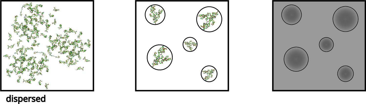
A schematic showcasing the process of liquid-liquid phase separation of α-synuclein (αS).
Figure 2
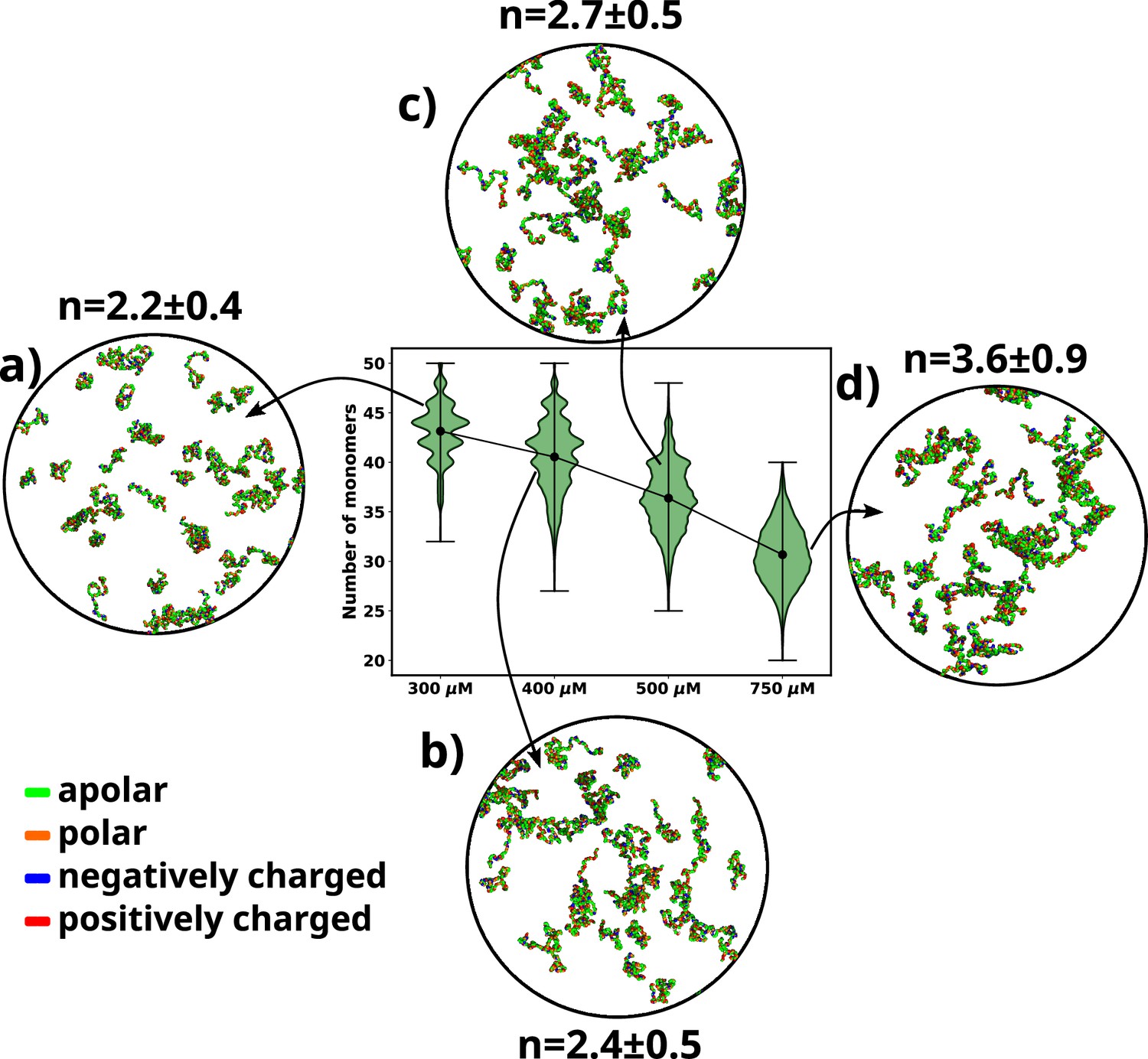
A violin plot showing the distribution of number of monomers present for different concentrations of α-syn.
The blue dot at the middle of each distribution represents the mean number of monomers observed for each concentration. For each concentration we show representative snapshots of the system. For each concentration, we also report the statistics of the number of chains in the largest cluster (n). (a) A snapshot from the simulation at 300 μM α-syn. (b) A snapshot from the simulation at 400 μM α-syn. (c) A snapshot from the simulation for 500 μM α-syn. (d) A snapshot from the simulation at 750 μM α-syn.
Figure 3
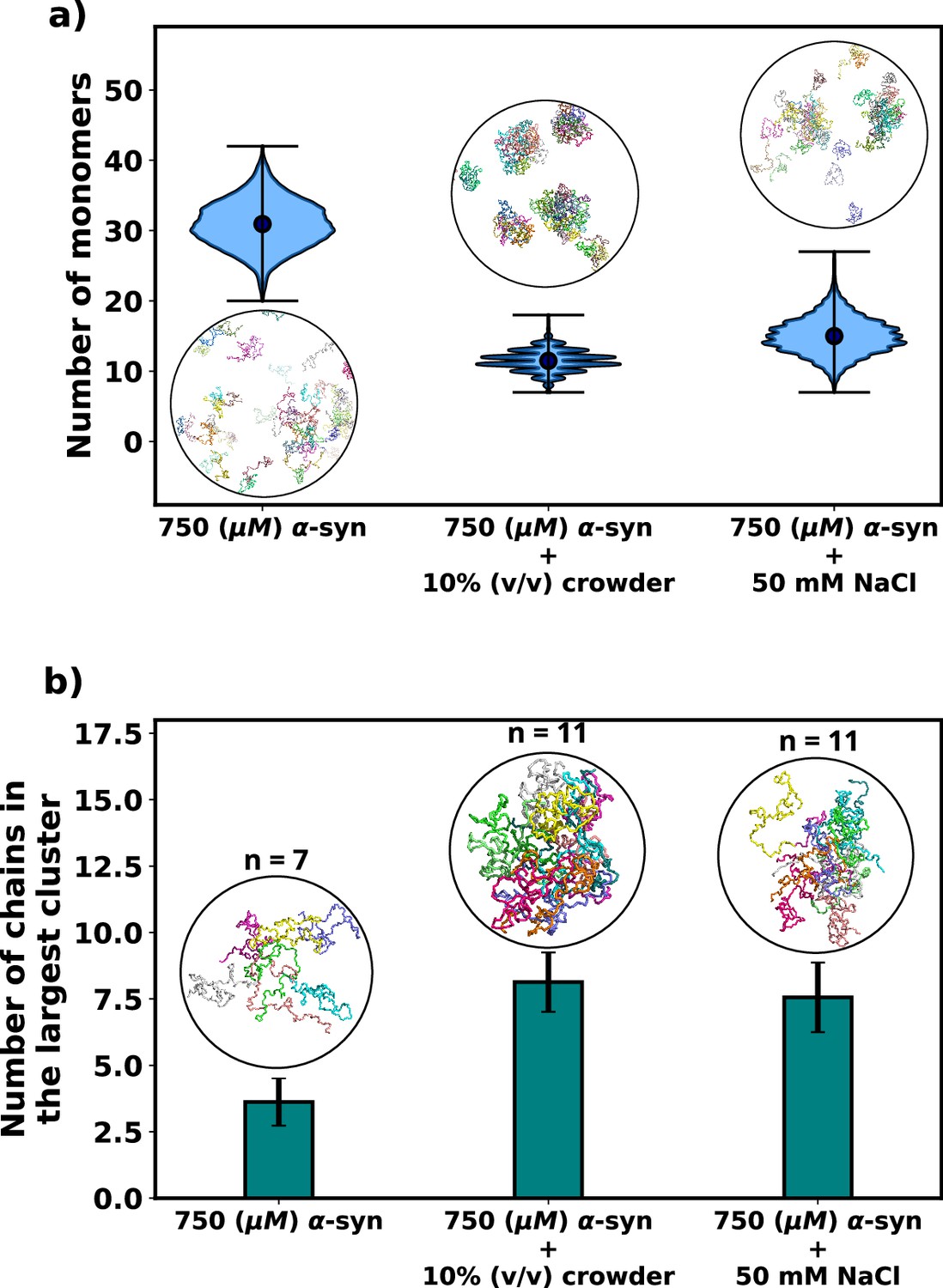
Effect of salt and crowder on αS aggregation.
(a) A violin plot showing the distribution of the number of monomers for α-syn at 750 μM without and with crowder. The blue dots represent the means of each distribution. The snapshots represent the extent aggregation for a visual comparison. (b) A bar plot showing the number of chain in the largest cluster formed by α-syn at 750 μM without and with crowder. The snapshots show the largest cluster formed for each scenario.
Figure 4 with 1 supplement
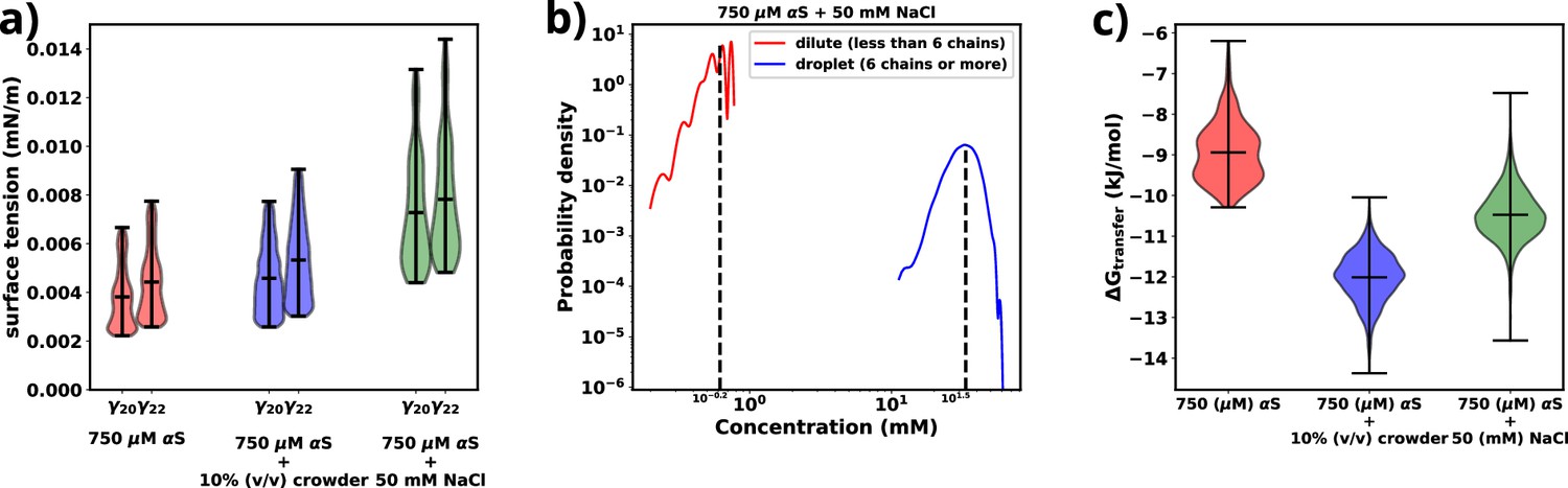
Exploring energetics of αS aggregation.
(a) Surface tensions of droplets, estimated from and , for three cases have been shown. Both and provide almost similar estimates of the value of surface. (b) Comparison of protein concentrations for the dilute (red) and the droplet (blue) phases for 750 μM αS+50 mM NaCl. (c) Excess free energy of transfer comparison for three cases.
Figure 4—figure supplement 1
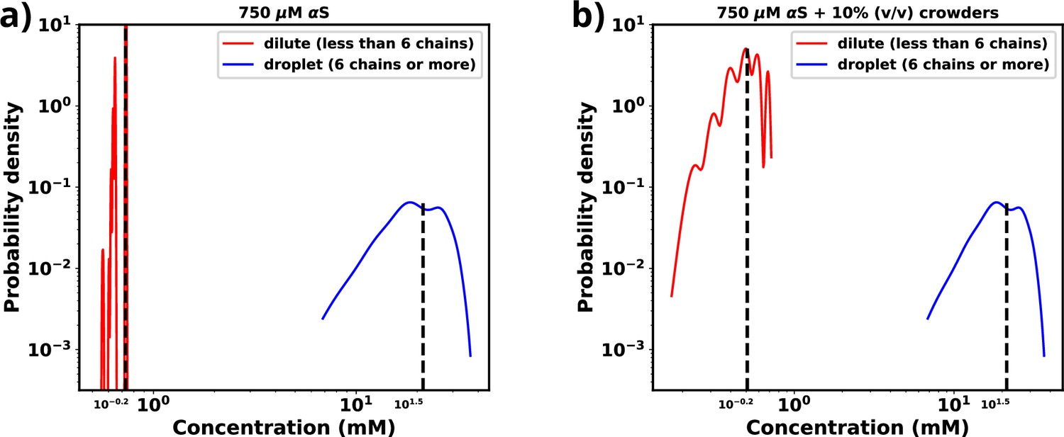
Comparison of protein concentration at two different phase.
(a) Comparison of protein concentrations in the dense and the dilute phase for 750 μM αS. (b) Comparison of protein concentrations in the dense and the dilute phase for 750 μM αS in the presence of 10% (vol/vol) crowders.
Figure 5 with 1 supplement
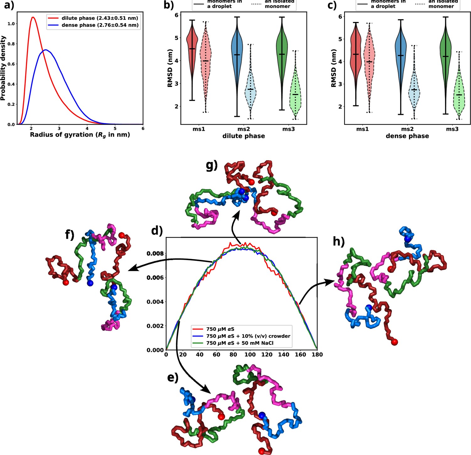
Exploring conformational change in αS monomers upon LLPS.
All the figures are for 750 μM αS+50 mM NaCl. (a) Distribution of Rg for proteins present in the dense or the dilute phases. (b) Comparison of root mean square deviation (RMSD) for protein chains present in the dilute phase, with single-chain RMSDs as the reference (dotted edges). (c) Comparison of RMSD for protein chains present in the dense phase, with single-chain RMSDs as the reference (dotted edges). (d) Distribution of the angle of orientation of two chains inside the droplet for the three different scenarios. (e) Representative snapshot for angle between 0 and 20 degree. (f) Representative snapshot for angle between 50 and 70 degree. (g) Representative snapshot for angle between 80 and 120 degree. (h) Representative snapshot for angle between 150 and 180 degree.
Figure 5—figure supplement 1
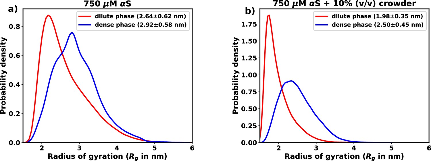
Comparison of monomer size in in liquid and dense phase.
(a) Comparison of in the dense and the dilute phase for 750 μM α-synuclein (αS). (b) Comparison of in the dense and the dilute phase for 750 μM αS in the presence of 10% (vol/vol) crowders.
Figure 6 with 3 supplements
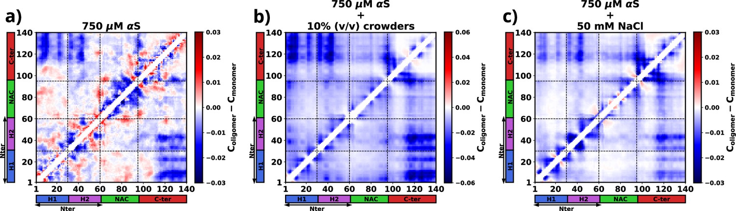
The figure presents the residue-wise, intra-protein difference contact maps where the average contact probability of monomers in the dilute phase was subtracted from the average contact probability of monomers in the dense/droplet phase for three cases.
(a) 750 μM α-synuclein (αS) in water. (b) 750 μM αS in the presence of 10% (vol/vol) crowders. (c) 750 μM αS in the presence of 50 mM NaCl.
Figure 6—figure supplement 1
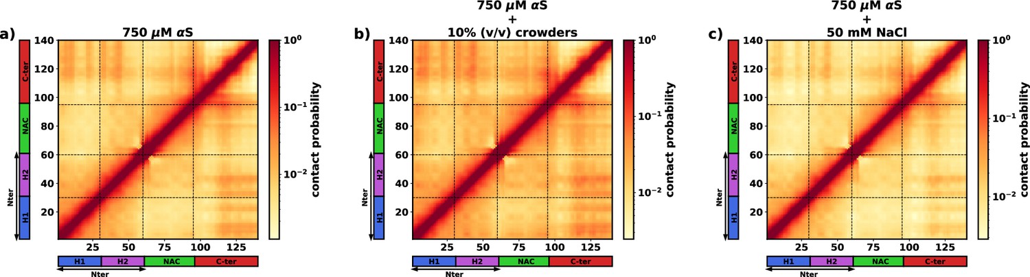
The intra-protein contact probability heatmap for proteins in the dilute phase for three scenarios.
(a) 750 μM αS. (b) 750 μM α-synuclein (αS) + 10% (vol/vol) crowders. (c) 750 μM αS + 50 mM NaCl.
Figure 6—figure supplement 2
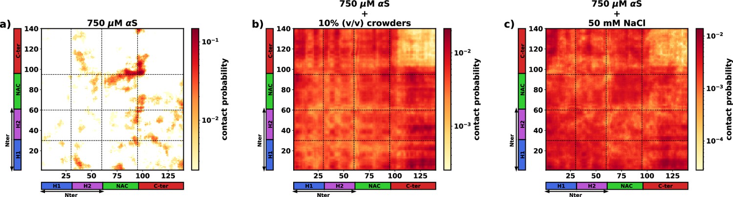
The inter-protein contact probability heatmap for proteins in the dense phase for three scenarios.
(a) 750 μM αS. (b) 750 μM αS + 10% (vol/vol) crowders. (c) 750 μM αS + 50 mM NaCl.
Figure 6—figure supplement 3
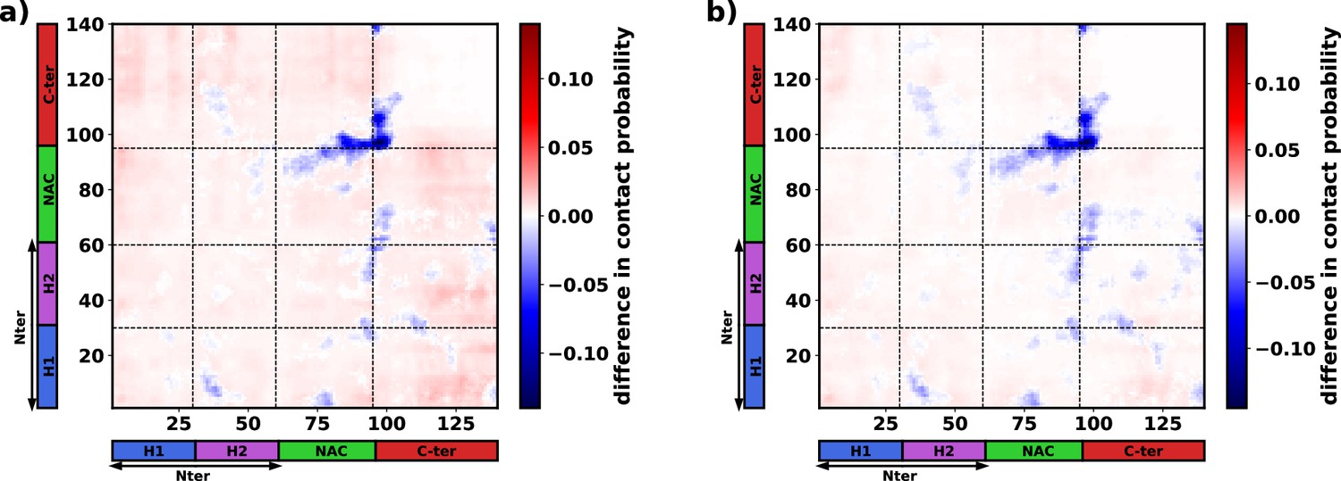
The difference in inter-protein contact probabilities heatmap for proteins in the dense phase.
(a) 750 μM αS + 10% (vol/vol) crowders - 750 μM αS. (b) 750 μM αS + 50 mM NaCl - 750 μM αS.
Figure 7
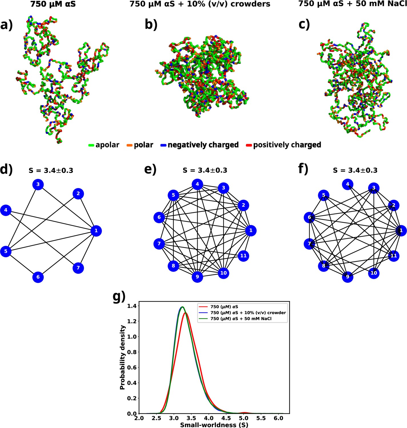
A graph theoretic analysis to characterize the "connectedness" of aS chains inside a droplet.
(a) The largest cluster formed by αS at 750 μM. (b) The largest cluster formed by αS at 750 μM in the presence of 10% (vol/vol) crowder. (c) The largest cluster formed by αS at 750 μM in the presence of 50 mM salt. Different residues have been color coded as per the figure legend. (d) A graph showing the contacts among different chains constituting the largest cluster formed by αS at 750 μM. (e) A graph showing the contacts among different chains constituting the largest cluster formed by αS at 750 μM in the presence of 10% (vol/vol) crowder. (f) A graph showing the contacts among different chains constituting the largest cluster formed by αS at 750 μM in the presence of 50 mM NaCl. The mean small-worldness (S) of all droplet has been reported above the graph. (g) Distribution of small-worldness (S) for all scenarios.
Figure 8
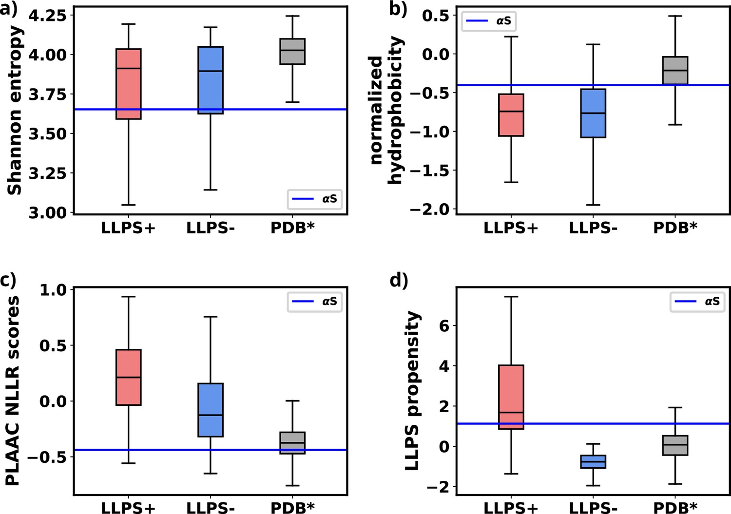
Comparison of primary sequence derived features for various datasets and aS.
(a) Comparison of Shannon entropy of different datasets with αS. (b) Comparison of Kyte-Doolittle hydrophobicity of different datasets with αS. (c) Comparison of LLR scores, obtained from PLAAC, of different datasets with αS. (d) Comparison of liquid-liquid phase separation (LLPS) propensity scores, obtained from catGRANULE websever, of different datasets with αS. The values have been summarized in Figure 8—source data 5.
-
Figure 8—source data 1
Shannon entropy (Shannon, 1948) for various datasets and α-synuclein (αS).
- https://cdn.elifesciences.org/articles/95180/elife-95180-fig8-data1-v1.docx
-
Figure 8—source data 2
Normalized Kyte-Doolittle hydrophobicity (Kyte and Doolittle, 1982) scores for various datasets and α-synuclein (αS).
- https://cdn.elifesciences.org/articles/95180/elife-95180-fig8-data2-v1.docx
-
Figure 8—source data 3
PLAAC normalized, maximum of the sum of PLAAC log-likelihood ratios (NLLR) (Lancaster et al., 2014) scores for various datasets and α-synuclein (αS).
- https://cdn.elifesciences.org/articles/95180/elife-95180-fig8-data3-v1.docx
-
Figure 8—source data 4
catGRANULE (Bolognesi et al., 2016) scores for various datasets and α-synuclein (αS).
- https://cdn.elifesciences.org/articles/95180/elife-95180-fig8-data4-v1.docx
-
Figure 8—source data 5
Comparison of primary sequence derived features for various datasets and α-synuclein (αS).
- https://cdn.elifesciences.org/articles/95180/elife-95180-fig8-data5-v1.docx
Figure 9
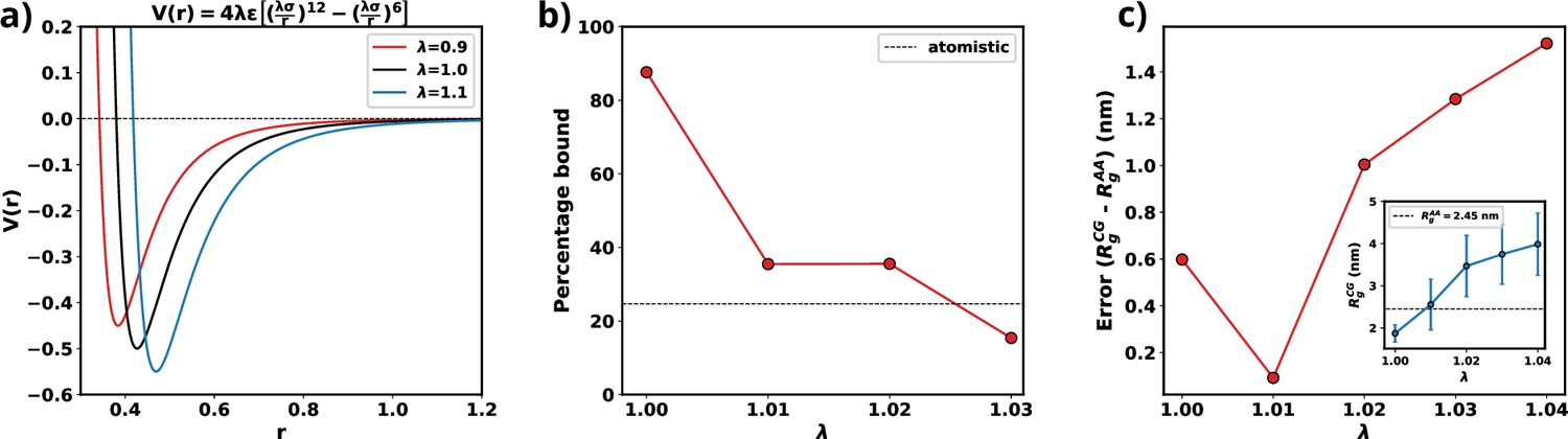
Optimization of Martini 3 water-protein interactions to tailor the forcefield for αS.
(a) Plot of LJ potentials with respect to . (b) The percentage bound values between two coarse-grained (CG) αS chains for different values of . The dashed black line represents the percentage bound values for two all-atom chains. (c) Error between calculated from CG and from all-atom simulations vs . The inset plot showcases the average values of obtained from CG along with their respective standard deviations. The dashed line represents the average value from all-atom simulations.
Figure 10

Mean squared displacements (MSD) vs time plots for different values of α.
The black line represents the MSD obtained from atomistic simulations with purely repulsive fullerene-fullerene interactions.
Figure 11
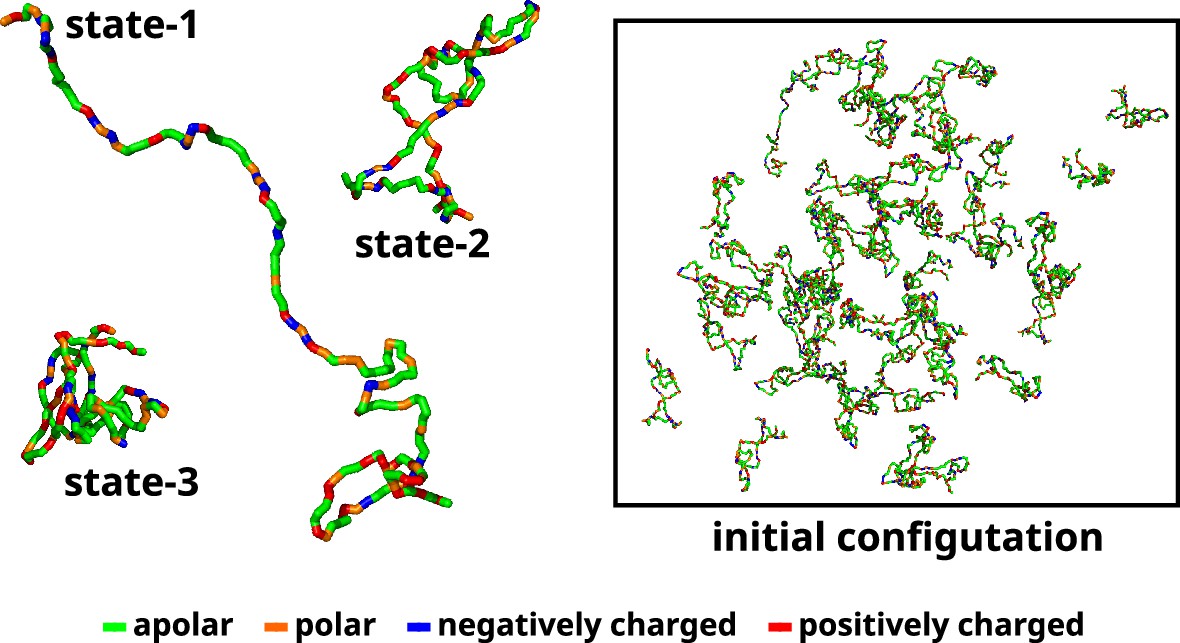
Initial configuration of αS for all multi-chain CG simulations.
The left side of the figure shows the coarse-grained representation of three different conformation of αS. State-1 is the most extended conformation, followed by state-2 and finally state-3 which is the most compact conformation. The right side of the figure shows the mixture of all these conformations with a total of 50 chains in a cubic box. The residues have been color coded on the basis of their polarity/charge.
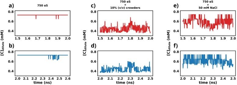
Figure 12 with 1 supplement
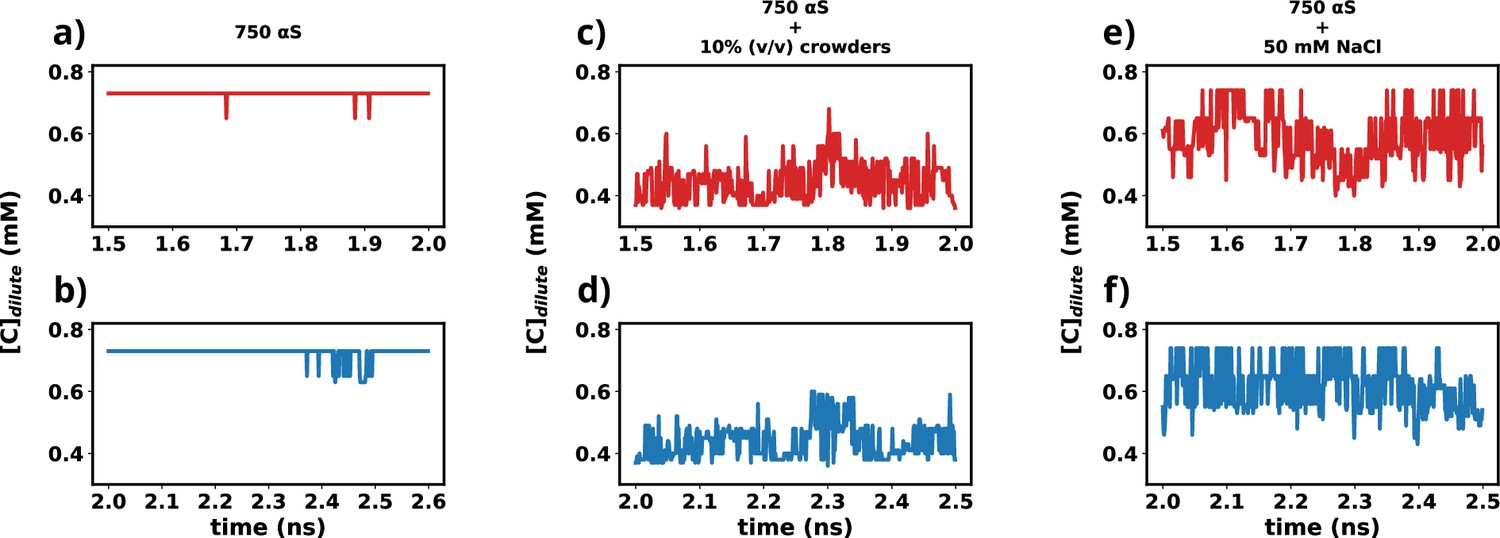
Time profiles of different metrics that showcase the attainment of steady state.
(a) Concentration vs time profile of αS between 1.5 and 2.0 μs. (b) Concentration vs time profile of αS between 2.0 and 2.5 μs. (c) Concentration vs time profile of αS + 10% (vol/vol) crowders between 1.5 and 2.0 μs. (d) Concentration vs time profile of αS + 10% (vol/vol) crowders between 2.0 and 2.5 μs. (e) Concentration vs time profile of αS + 50 mM NaCl between 1.5 and 2.0 μs. (f) Concentration vs time profile of αS + 50 mM NaCl between 2.0 and 2.5 μs.
Figure 12—figure supplement 1
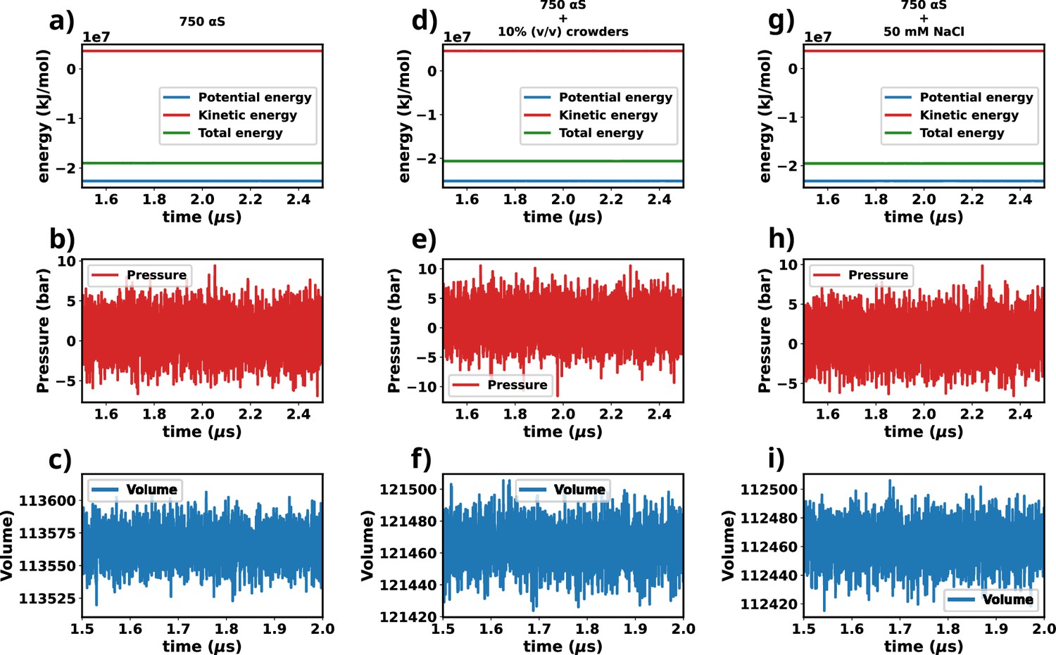
Assesment of equilibration of simulated trajectories.
(a–c) Energies, pressure, and volume of the simulation box for 750 μM α-synuclein (αS). (d–f) Energies, pressure, and volume of the simulation box for 750 μM αS + 10% (vol/vol) crowders. (g–i) Energies, pressure, and volume of the simulation box for 750 μM αS + 50 mM NaCl.
Author response image 1
Author response image 2

Tables
Table 1
Details of the systems that were explored.
| Summary | Conc. of αS (μM) | Box size (nm) | # water | # crowders | # Na+ | # Cl- |
|---|---|---|---|---|---|---|
| 300 μM αS in water | 300 | 65.66 | 2,304,122 | 0 | 450 | 0 |
| 400 μM αS in water | 400 | 59.69 | 1,729,213 | 0 | 450 | 0 |
| 500 μM αS in water | 500 | 55.52 | 1,389,721 | 0 | 450 | 0 |
| 750 μM αS in water | 750 | 48.42 | 920,023 | 0 | 450 | 0 |
| 750 μM αS + 10%(vol/vol) crowder | 750 | 48.42 | 843,011 | 20,128 | 450 | 0 |
| 750 μM αS + 50 mM NaCl | 750 | 48.42 | 913,357 | 0 | 3783 | 3333 |
-
For all simulations, a total of 50 monomeric protein chains have been used which comprise 1×ms1, 45×ms2, and 4×ms3.
Table 2
Runtimes of different simulations.
| System | No. of replicas | Runtime (s) |
|---|---|---|
| 300 μM αS | 1 | 2.5 μs |
| 400 μM αS | 1 | 4.3 μs |
| 500 μM αS | 1 | 4.1 μs |
| 750 μM αS | 4 | 2.6, 3.1, 3.0, 3.5 μs |
| 750 μM αS + 10% (vol/vol) crowders | 4 | 2.8, 2.5, 2.6, 2.6 μs |
| 750 μM αS + 50 mM NaCI | 4 | 2.6, 2.4, 2.6, 2.3 μs |
Additional files
Download links
A two-part list of links to download the article, or parts of the article, in various formats.
Downloads (link to download the article as PDF)
Open citations (links to open the citations from this article in various online reference manager services)
Cite this article (links to download the citations from this article in formats compatible with various reference manager tools)
Modulation of α-synuclein aggregation amid diverse environmental perturbation
eLife 13:RP95180.
https://doi.org/10.7554/eLife.95180.3


