Figures and data in The recurrent temporal restricted Boltzmann machine captures neural assembly dynamics in whole-brain activity | eLife

Figures
Additional files

4 figures and 1 additional file

Figures

Figure 1

Download asset Open asset

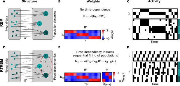
The recurrent temporal RBM (RTRBM) extends the restricted Boltzmann machine (RBM) by additionally accounting for temporal interactions of the neural assemblies.

(A) A schematic depiction of an RBM with visible units (neurons) on the left, and hidden units (neural assemblies) on the right. The visible and hidden units are connected through a set of weights $W$ . (B) An example $W$ matrix where a subset of visible units is connected to one hidden unit. Details of the equations in panel B and E are given in Materials and methods. (C) Hidden and visible activity traces were generated by sampling from the RBM. Due to its static nature, the RBM samples do not exhibit any sequential activation pattern, but merely show a stochastic exploration of the population activity patterns. (D) Schematic depiction of an RTRBM. The RTRBM formulation matches the static connectivity of the RBM, but extends it with the weight matrix $U$ to model temporal dependencies between the hidden units. (E) In the present example, assembly 1 excites assembly 2, assembly 2 excites assembly 3, and assembly 3 excites assembly 1, while the remaining connections were set to 0. (F) Hidden and visible activity traces were generated by sampling from the RTRBM. In contrast to the RBM samples, the RTRBM generates samples featuring a sequential firing pattern. It is able to do so due to the temporal weight matrix $U$ which enables modeling temporal dependencies.

Figure 2 with 1 supplement

Download asset Open asset

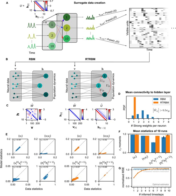
The recurrent temporal RBM (RTRBM) outperforms the restricted Boltzmann machine (RBM) on sequential statistics on simulated data.

(A) Simulated data generation: Hidden Units ( $N_{h}$ ) interact over time to generate firing rate traces which are used to sample a Poisson train. For example, assembly 1 drives assembly 2 and inhibits assembly 10, both at a single time-step delay. (B) Schematic depiction of the RBM and RTRBM trained on the simulated data. (C) For the RBM, the aligned estimated weight matrix $\hat{W}$ contains spurious off-diagonal weights, while the RTRBM identifies the correct diagonal structure (top). For the assembly weights $U$ (left), the RTRBM also converges to similar aligned estimated temporal weights $\hat{U}$ (right). (D) The RTRBM attributes only a single strong weight to each visible unit (( $w_{i, j} > 0.5 σ$ , where $σ$ is the standard deviation of $W$ )), consistent with the specification in $W$ , while in the RBM multiple significant weights get assigned per visible units. (E) The RBM and RTRBM perform similarly for concurrent ( $⟨ v_{i} ⟩$ , $⟨ v_{i} v_{j} ⟩$ ) statistics, but the RTRBM provides more accurate estimates for sequential ( $⟨ v_{i}^{[t]} v_{j}^{[t + 1]} ⟩$ , $⟨ h_{i}^{[t]} h_{j}^{[t + 1]} ⟩$ ) statistics. In all panels, the abscissa refers to the data statistics in the test set, while the ordinate shows data sampled from the two models,, respectively. (F) The trained RTRBM and the RBM yield similar concurrent moments, but the RTRBM significantly outperformed the RBM on time-shifted moments (see text for details on statistics). (G) The RTRBM achieved significantly lower normalized mean squared error (nMSE) when predicting ahead in time from the current state in comparison to RBMs for up to four time-steps.

Figure 2—figure supplement 1

Download asset Open asset

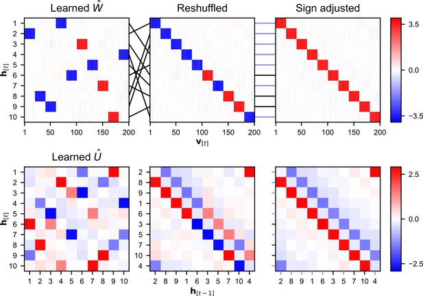
Alignment of weight matrices after learning.

An alignment procedure is used to be able to enable comparison between the estimated temporal weight matrix $\hat{U}$ and the original temporal matrix used to generate the data. Details on the alignment procedure can be found in alignment of the estimated temporal weight matrix. (A) The link between hidden units and assemblies of visible units can often be clearly identified within the weight matrix, making it possible to define an ordering of the hidden units such that it is in line with the ordering of the assemblies. This leads to a shuffling of the rows in the $\hat{W}$ matrix. The sign of the mean weight between an assembly and its matched hidden unit is used to identify inverse relations. (B) The reordering of the hidden units leads to a reshuffling of both the rows and the columns of the $\hat{U}$ matrix. The sign of an entry is switched when the two hidden units have an opposing sign to their matched assembly of visible units.

Figure 3

Download asset Open asset

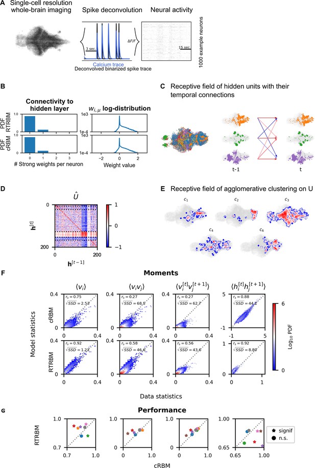
Recurrent temporal RBM (RTRBM) often outperforms the compositional restricted Boltzmann machine (cRBM) on zebrafish data.

(A) Whole-brain neural activity of larval zebrafish was imaged via Calcium-indicators using light-sheet microscopy at single neuron resolution (left). Calcium activity (middle, blue) is deconvolved by blind, sparse deconvolution to obtain a binarized spike train (middle, black). The binarized neural activity of 1000 randomly chosen neurons (right). (B) Left: Distribution of all visible-to-hidden weights. Here, a strong weight is determined by proportional thresholding, $w_{i, j} > w_{t h r}$ . Here $w_{t h r}$ is set such that 5000 neurons have a strong connection towards the hidden layer. Right: log-weight distribution of the visible to hidden connectivity. (C) The RTRBM extracts sample assemblies (color indicates assembly) by selecting neurons based on the previously mentioned threshold. Visible units with stronger connections than this threshold for a given hidden unit are included. Temporal connections (inhibitory: blue, excitatory: red) between assemblies are depicted across time-steps. (D) Temporal connections between the assemblies are sorted by agglomerative clustering (dashed lines separate clusters, colormap is clamped to $[- 1, 1]$ ). Details on the clustering method can be found in Materials and methods. (E) Corresponding receptive fields of the clusters identified in (D), where the visible units with strong weights are selected similarly to (B). The receptive field of cluster 5 has been left out as it contains only a very small number of neurons with strong weights based on the proportional threshold. (F) Comparative analysis between the cRBM (bottom row) and RTRBM (top row) on inferred model statistics and data statistics (test dataset). Compared in terms of Spearman correlations and sum square difference. From left to right: the RTRBM significantly outperformed the cRBM on the mean activations $⟨ v_{i} ⟩$ ( $p < ϵ$ ), pairwise neuron-neuron interactions $⟨ v_{i} v_{j} ⟩$ ( $p < ϵ$ ), time-shifted pairwise neuron-neuron interactions $⟨ v_{i}^{[t]} v_{j}^{[t + 1]} ⟩$ ( $p < ϵ$ ), and time-shifted pairwise hidden-hidden interactions $⟨ h_{i}^{[t]} h_{j}^{[t + 1]} ⟩$ ( $p < ϵ$ ) for example fish 4. (G) The methodology in panel F is extended to analyze datasets from eight individual fish, each color representing one individual fish. Spearman correlation and the assessment of significant differences between both models are determined using a bootstrap method (see Materials and methods for details).

Figure 4

Download asset Open asset

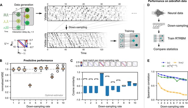
Neural interaction timescale can be identified via recurrent temporal RBM (RTRBM) estimates over multiple timescales.

(A) Training paradigm. Simulated data is generated as in Figure 2, but with temporal interactions between populations at a delay of $Δ t_{A} = 4$ time-steps. This data is downsampled according to a downsampling rate $Δ t_{D}$ by taking every $Δ t_{D}$ -th time-step (shown here is $Δ t_{D} = 4$ ), and used for training different RTRBMs. (B) Performance of the RTRBM for various down-sampling rates measured as the normalized mean squared error (MSE) in predicting the visible units one time-step ahead ( $N = 10$ models per $Δ t_{D}$ ). Dotted line shows the mean estimate of the lower bound ± SEM ( $N = 10,000$ ) due to inherent variance in the way the data is generated (see Materials and methods). Dashed gray line indicates the theoretical performance of an uninformed, unbiased estimator $P ({\hat{v}}_{i}^{t} = 1) = ⟨ v_{i} ⟩$ . (C) Cosine similarity between the interaction matrix $U$ and the aligned learned matrices $\hat{U}$ , both z-scored. Bars and errorbars show mean and standard deviation, respectively, across the $N = 10$ models per $Δ t_{D}$ . Dark lines show absolute values of the mean cosine similarity. Shown above are the $\hat{U}$ matrices with the largest absolute cosine similarity per down-sampling rate. (D) The same procedure as in (A) is performed on neural data in order to find the effect of down-sampling here. (E) Spearman correlation of three important model statistics across different down-sampling rates for neural data from example fish 4, similar to Figure 3F. Dots and shaded areas indicate mean and two times standard deviation, determined using a bootstrap method (see Materials and methods for details).

Additional files

MDAR checklist: https://cdn.elifesciences.org/articles/98489/elife-98489-mdarchecklist1-v1.pdf
Download elife-98489-mdarchecklist1-v1.pdf

Download links

A two-part list of links to download the article, or parts of the article, in various formats.

Downloads (link to download the article as PDF)

Open citations (links to open the citations from this article in various online reference manager services)

Mendeley

Cite this article (links to download the citations from this article in formats compatible with various reference manager tools)

Sebastian Quiroz Monnens
Casper Peters
Luuk Willem Hesselink
Kasper Smeets
Bernhard Englitz

(2024)

The recurrent temporal restricted Boltzmann machine captures neural assembly dynamics in whole-brain activity

eLife 13:RP98489.

https://doi.org/10.7554/eLife.98489.3

Sign up for email alerts

Privacy notice