ATP binding facilitates target search of SWR1 chromatin remodeler by promoting one-dimensional diffusion on DNA
- Department of Biophysics and Biophysical Chemistry, Johns Hopkins University, United States
- Department of Biology, Johns Hopkins University, United States
- Howard Hughes Medical Institute, United States
- Johns Hopkins University, Department of Biomedical Engineering, United States
- Johns Hopkins University, Department of Biophysics, United States
Figures
Figure 1 with 1 supplement
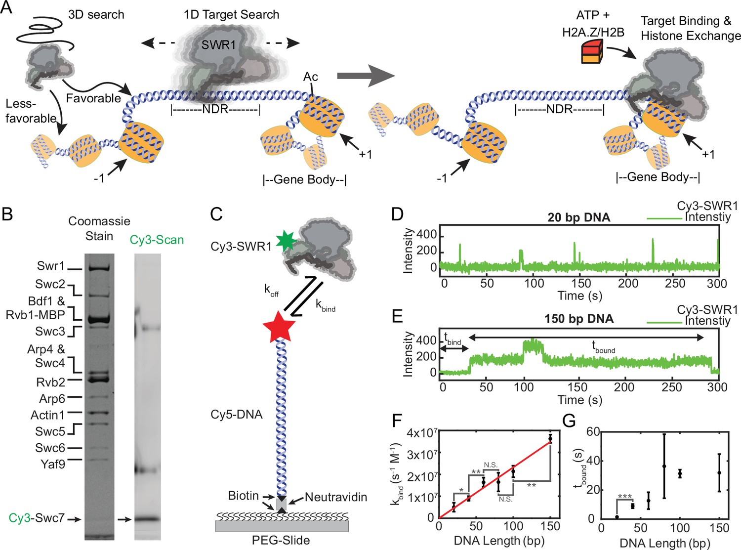
SWR1 binds DNA in short- and long-lived states and prefers longer DNAs.
(A) Proposed facilitated search mechanism for how SWR1 locates the +1 nucleosome. (B) A denaturing sodium dodecyl sulfate–polyacrylamide gel electrophoresis (SDS–PAGE) of reconstituted Cy3-SWR1 imaged for Coomassie (left) and Cy3 fluorescence (right). Cy3-Swc7 is faint when stained with Coomassie but is a prominent band in the Cy3 scan. The two diffuse bands that run at higher molecular weight and appear in the Cy3 scan are carry over from the ladder loaded in the adjacent lane. (C) A schematic of the single-molecule colocalization experiment used for kinetic measurements of Cy3-SWR1 binding to Cy5-labeled DNA of different lengths. Representative traces of Cy3-SWR1 binding to (D) 20 bp Cy5-DNA and to (E) 150 bp Cy5-DNA. A second Cy3-SWR1 can be seen binding at approximately 100 s. (F) The on-rate binding constant for the initial binding event, (kbind) for SWR1 to DNA of different lengths, error bars are standard deviation. N values: 20 bp (40), 40 bp (67), 60 bp (267), 80 bp (129), 100 bp (221), 150 bp (409). The red line is a linear fit to the data, where R2 = 0.99 [two technical replicates represented, statistical differences determine via Student’s t-test, where asterisks indicate the level of significance as conventionally defined (* = p < 0.05; ** = p < 0.01, *** = p < 0.001, n.s. = not significant)]. (G) The lifetime (tbound) of Cy3-SWR1 bound to DNAs of different lengths, error bars are standard deviation. N values: 20 bp (48), 40 bp (118), 60 bp (291), 80 bp (382), 100 bp (339), 150 bp (363) [two technical replicates represented, statistical differences determine via Student’s t-test, where asterisks indicate the level of significance as conventionally defined].
-
Figure 1—source data 1
Numerical data and statistics underlying panels F and G.
- https://cdn.elifesciences.org/articles/77352/elife-77352-fig1-data1-v2.zip
-
Figure 1—source data 2
Gel images (Coomassie and Cy3 scans) shown in panel B.
- https://cdn.elifesciences.org/articles/77352/elife-77352-fig1-data2-v2.zip
Figure 1—figure supplement 1
Cy3-SWR1 purification and DNA-binding kinetics.
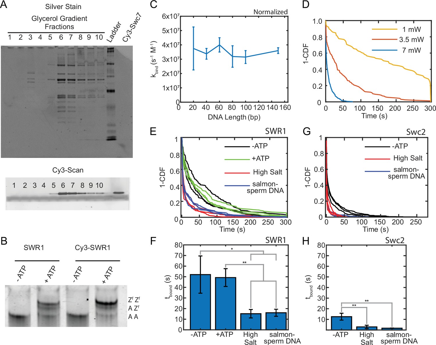
(A) A glycerol gradient purification of the Cy3–SWR1 complex after Cy3-Swc7 reincorporation. A silver stain (top image) shows that the SWR1 complex eluted in fractions 6 and 7 of the gradient. A Cy3 scan of the same gel shows that Cy3-Swc7 is also found in fractions 6 and 7 (confirmed by a Cy3-Swc7 only control at the end of the gel). This demonstrates that the Cy3-Swc7 is incorporated into the SWR1ΔSwc7 complex. (B) A histone exchange assay that shows Cy3-SWR1 (right lanes) is as active as the unlabeled wild-type SWR1 complex. The gel shift is caused by the incorporation of triple flag-tagged ZB dimers (denoted Zf) into the nucleosome (AB dimer denoted with a letter A). (C) Normalized plot shown in Figure 1F of kbind. Values and errors are normalized to the longest DNA tested; values are divided by the quotient of the length of DNA divided by 150 bp. No statistical difference between DNA lengths as assessed using a Student’s t-test. (D) tbound for Cy3-SWR1 bound to 150 bp DNA measured at different laser powers. N values: 7 W (154), 3.5 W (139), 1 W (88) [one technical replicate represented]. (E) 1-CDF for Cy3-SWR1 bound to 150 bp DNA in histone exchange reaction buffer without ATP, with 1 mM ATP, with 200 mM NaCl, or with 0.2 µg/ml of salmon sperm DNA [three technical replicates]. (F) Quantification of panel E; tbound for Cy3-SWR1 bound to 150 bp DNA with error bars representing standard deviation for the different conditions. N values: buffer + ATP (588), buffer only (563), high salt (538), salmon sperm DNA (750) [three technical replicates represented, statistical differences determine via Student’s t-test, where asterisks indicate the level of significance as conventionally defined (* = p < 0.05; ** = p < 0.01)]. (G) 1-CDF for Cy3-Swc2 bound to 150 bp DNA in histone exchange reaction buffer without ATP, with 200 mM NaCl or with 0.2 µg/m of salmon sperm DNA [three technical replicates per condition represented; all data are shown] (H) Quantification of panel G; tbound for Cy3-Swc2 bound to 150 bp DNA with error bars representing standard deviation for the different conditions. N values: buffer only (1027), high salt (605), salmon sperm DNA (699) [three technical replicates; statistical differences determine via Student’s t-test]. (E, G) 1-CDF plots for both SWR1 and Swc2 binding to 150 bp DNA under all conditions tested were best fit to double exponential decay functions. (F, H) tbound values are amplitude averages which normalize the reported tbound based on the relative contribution of the short- versus long-lived tau to the fit data. While the short tau values are reported as part of the amplitude averages, for C-Trap experiments, the long tau is the more relevant value as very short-lived binding events are not easily observed in our C-Trap setup. The overall trends in tau-slow are consistent with the reported amplitude averages.
-
Figure 1—figure supplement 1—source data 1
Gel images (Coomassie and Cy3 scans) shown in panels A and B.
- https://cdn.elifesciences.org/articles/77352/elife-77352-fig1-figsupp1-data1-v2.zip
-
Figure 1—figure supplement 1—source data 2
Excel file corresponding to panels C, F, and H.
- https://cdn.elifesciences.org/articles/77352/elife-77352-fig1-figsupp1-data2-v2.zip
Figure 2 with 1 supplement
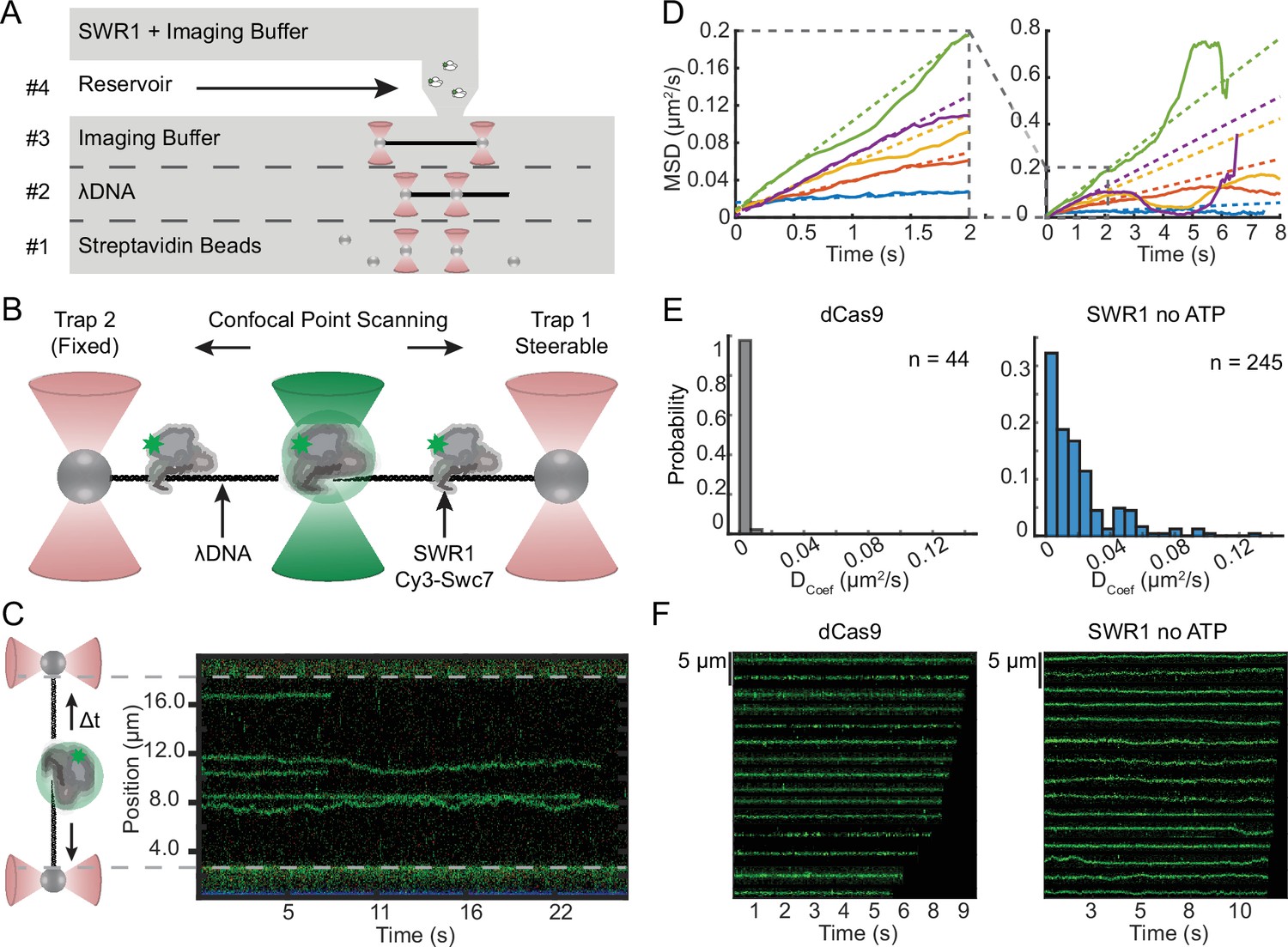
SWR1 diffuses on extended dsDNA.
(A) Schematic representation of a C-Trap microfluidics imaging chamber with experimental workflow depicted therein: #1 catch beads, #2 catch DNA, #3 verify single tether, and #4 image SWR1 bound to DNA. (B) Schematic representation of confocal point scanning across the length of lambda DNA tethered between two optically trapped beads. This method is used to monitor the position of fluorescently labeled SWR1 bound to DNA. (C) Example kymograph with a side-by-side schematic aiding in the interpretation of the kymograph orientation. (D) Mean squared displacement (MSD) versus time for a random subset of SWR1 traces in which no ATP is added. An enlargement of the initial linear portion is shown to the left where colored dashed lines are linear fits to this portion. (E) Histogram of diffusion coefficients for dCas9 (left) and SWR1 in which no ATP is added (right). (F) Segmented traces of dCas9 (left) and SWR1 in which no ATP is added (right).
-
Figure 2—source data 1
Data underlying panels D and E.
- https://cdn.elifesciences.org/articles/77352/elife-77352-fig2-data1-v2.zip
-
Figure 2—source data 2
Uncropped kymograph Tiff image from panel C.
- https://cdn.elifesciences.org/articles/77352/elife-77352-fig2-data2-v2.zip
Figure 2—figure supplement 1
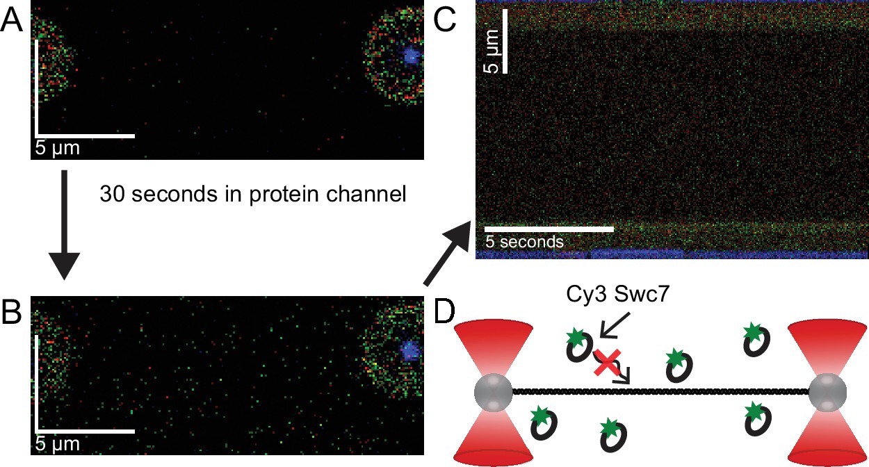
Cy3-Swc7 does not bind DNA without the SWR1 complex.
(A) A scan of lambda DNA pulled to 5 pN of tension in the absence of Cy3-labeled Swc7 imaged with green excitation. (B) A scan of lambda DNA in Cy3-Swc7 protein channel. Protein solution was flowed briefly to refresh the protein solution in the channel before and while DNA is introduced into the channel. The amount of Cy3-labeled Swc7 is equimolar to what is used for SWR1 sliding experiments. Apart from increased background, there is no specific interaction of Cy3-Swc7 with the DNA alone. (C) A kymograph along the length of the lambda DNA at a time resolution of 0.05 s per line scan also shows no bound Cy3-Swc7. (D) Schematic summary: Cy3-Swc7 does not bind lambda DNA alone, even at the faster time resolution used to generate a kymograph.
-
Figure 2—figure supplement 1—source data 1
Raw scans and kymograph tiff files.
- https://cdn.elifesciences.org/articles/77352/elife-77352-fig2-figsupp1-data1-v2.zip
Figure 3
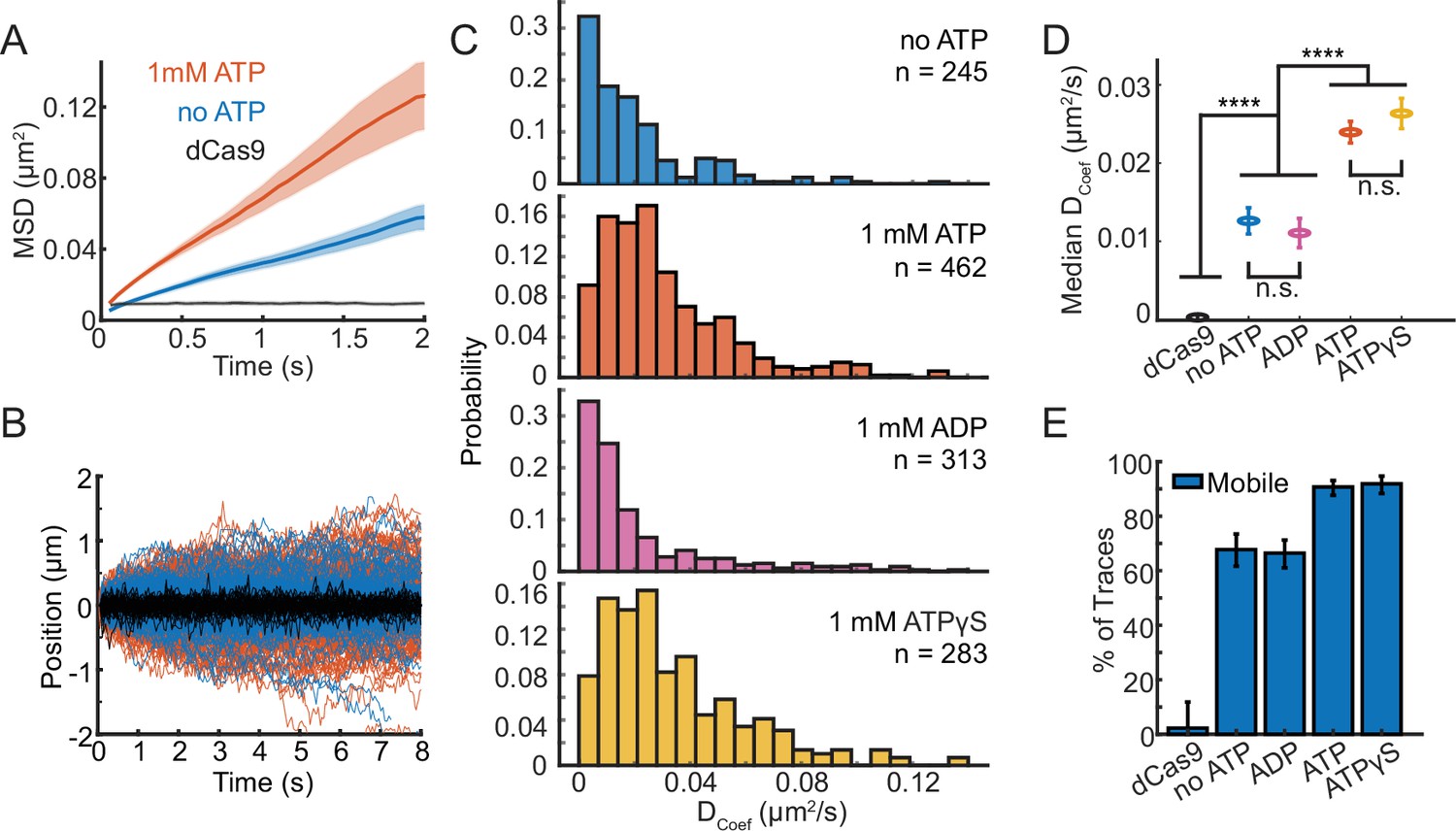
ATP binding modulates SWR1 diffusion.
(A) Mean squared displacement (MSD) versus time plotted for 1 mM ATP (orange, n = 124), no ATP (blue, n = 134), and dCas9 (black, n = 25) with shaded error bars standard error of the mean (SEM). (B) SWR1 trajectories aligned at their starts for 1 mM ATP (orange lines), no ATP (blue lines), and dCas9 as reference for immobility (black lines). All trajectories represented. (C) Histograms of diffusion coefficients extracted from individual trajectories for SWR1 diffusion in the presence of no ATP, 1 mM ATP, 1 mM ADP, and 1 mM ATPγS (from top to bottom). The number of molecules measured (n) for each condition is printed in each panel. (D) Median diffusion coefficients for SWR1 in varying nucleotide conditions. dCas9 is shown as a reference. Error bars are the uncertainty of the median. Statistical differences were determined via Student’s t-test, and asterisks indicate the level of significance (**** = p < 0.0001, n.s. = not significant). (E) Percentage of mobile traces in each condition, where immobility is defined as traces with similar diffusion coefficients to dCas9 (defined as diffusion coefficients smaller than 0.007 µm2/s). Error bars represent confidence intervals estimated using Matlab ‘bootci’ run with default settings and with a number of bootstrap samples = 5000, conditions with nonoverlapping error can be considered significantly different.
-
Figure 3—source data 1
Numerical data underlying panels A and C–E.
- https://cdn.elifesciences.org/articles/77352/elife-77352-fig3-data1-v2.zip
Figure 4 with 2 supplements
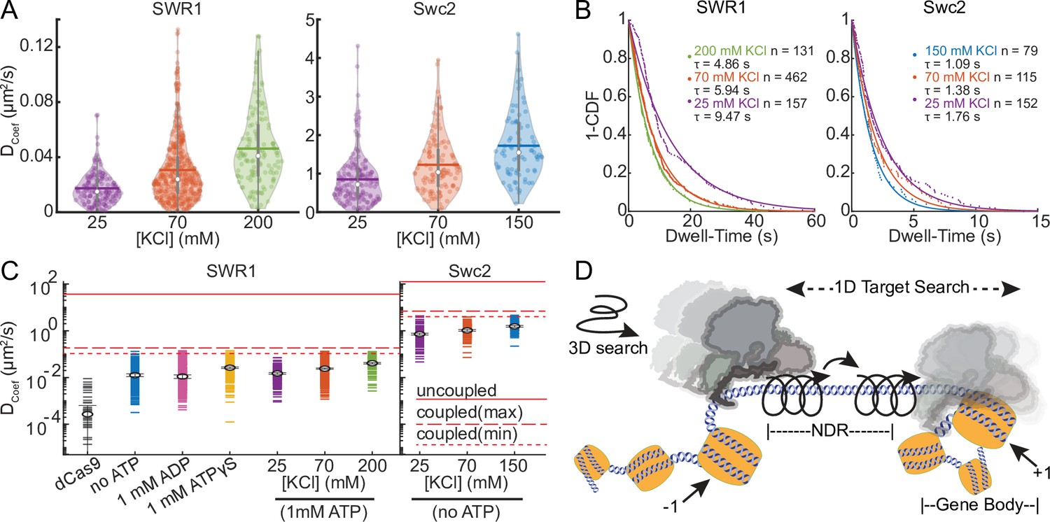
SWR1 and Swc2 DNA-binding domain (DBD) utilize a combination of sliding and hopping to scan DNA.
(A) Violin plots of diffusion coefficients for SWR1 and Swc2 DBD in increasing potassium chloride concentrations. Medians are shown as white circles and the mean is indicated with a thick horizontal line. 70 mM KCl represents the standard salt condition. (B) 1-CDF plots of SWR1 and Swc2 were fit to exponential decay functions to determine half-lives of binding in varying concentrations of potassium chloride. The number of molecules as well as half-lives determined is printed therein. Dots represent data points, while solid lines represent fits. Half-lives are calculated using the length of all the trajectories in each condition. (C) Upper limits for diffusion of SWR1 and Swc2 predicted using either a helically uncoupled model for hopping diffusion (uppermost solid red line) or a helically coupled model for sliding diffusion (lower dashed red lines). Two dashed lines are shown for helically coupled upper limits because the distance between the helical axis of DNA and the center of mass of either SWR1 or Swc2 is unknown. Markers represent median values. Dcoef values for each condition are shown as horizontal dashes, the number of molecules represented in each condition is as aforementioned. (D) A schematic representation of a model for how SWR1 likely performs 1D diffusion on DNA.
-
Figure 4—source data 1
Data underlying panels A–C.
- https://cdn.elifesciences.org/articles/77352/elife-77352-fig4-data1-v2.zip
Figure 4—figure supplement 1
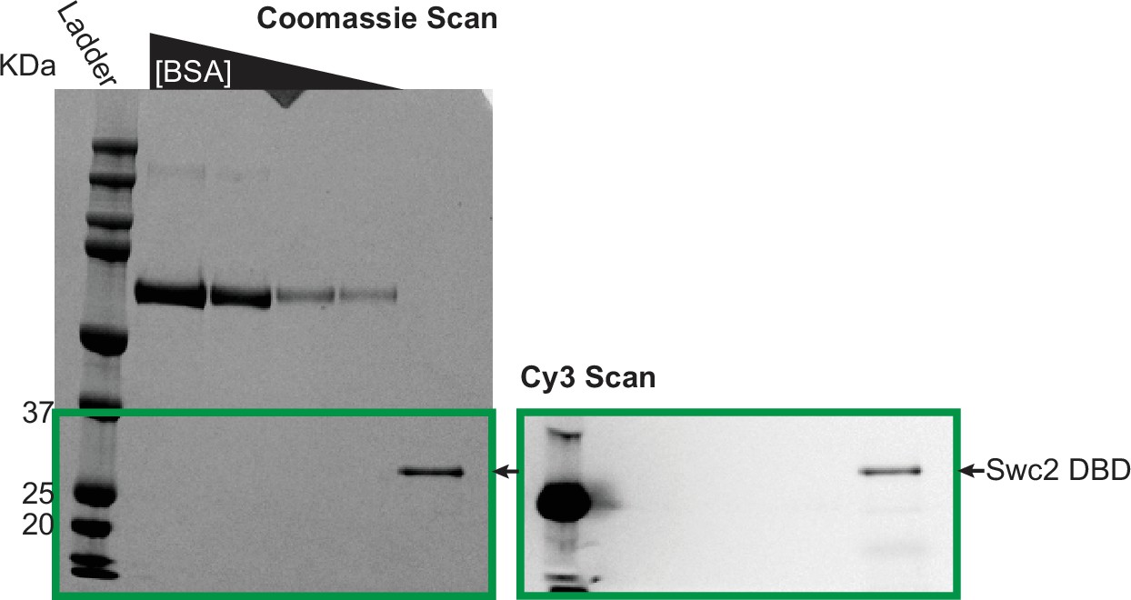
Purification and fluorophore labeling of the Swc2 DNA-binding domain (DBD).
Denaturing sodium dodecyl sulfate–polyacrylamide gel electrophoresis (SDS–PAGE) gel of the Swc2 DBD after nickel his-tag purification and labeling with Cy3-maleimide. A Cy3 scan of the gel (right) reveals that the Swc2 DBD (single band in Coomassie stain on the left) has been labeled with Cy3.
-
Figure 4—figure supplement 1—source data 1
Gel images (Coomassie and Cy3 scans).
- https://cdn.elifesciences.org/articles/77352/elife-77352-fig4-figsupp1-data1-v2.zip
Figure 4—figure supplement 2
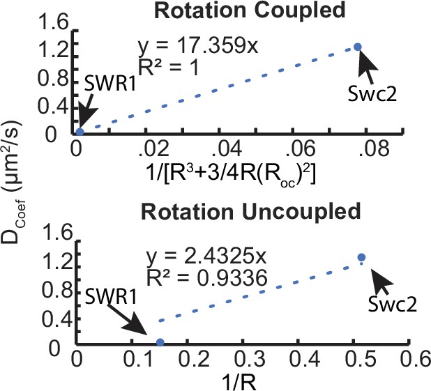
Rotation-coupled versus -uncoupled diffusion models and protein size effects on diffusion coefficient.
Apparent diffusion coefficient as a function of two relationships to the radius of SWR1 or Swc2 DNA-binding domain (DBD) where the protein size is printed below the graph and the corresponding model is stated above. A line passing through the origin is fit to both relationships, and the Pearson correlation coefficient is printed within the graph showing a slightly better fit of the measured diffusion coefficients to the rotation-coupled diffusion model.
Figure 5 with 1 supplement
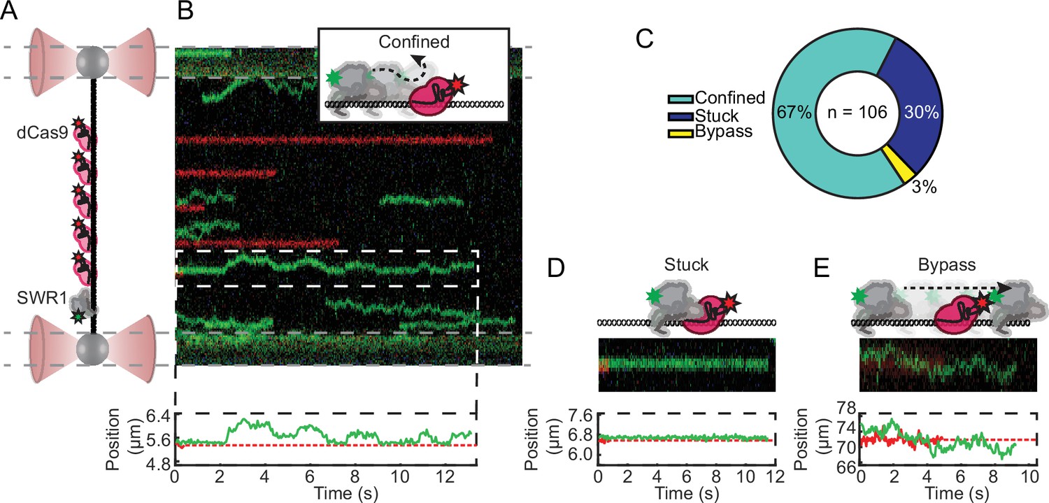
dCas9 protein roadblocks confine SWR1 1D diffusion.
(A) Schematic of the experimental setup: five Cy5-labeled gRNA position dCas9 at five evenly spaced sites along lambda DNA. Note that diffusion is measured in the presence of 1 mM ATP and standard salt conditions (70 mM KCl). (B) Example kymograph with five bound dCas9 in red, and an example of a confined diffusion encounter. Schematic, and single-particle tracking trajectory printed above and below. (C) Pie chart of the three types of colocalization events with the total number of observations printed therein. (D) Example of SWR1 stuck to the dCas9 within limits of detection; schematic, cropped kymograph, and single-particle tracking trajectory shown. Example of a SWR1-dCas9 bypass event; schematic, cropped kymograph, and single-particle tracking trajectory shown. (B, D, E) In the example single-particle tracking trajectory, dCas9 is represented as a dashed red line after Cy5 has photobleached, however due to long binding lifetimes of dCas9 we continue to use its position for colocalization analysis.
-
Figure 5—source data 1
All colocalization events with classifications indicated.
- https://cdn.elifesciences.org/articles/77352/elife-77352-fig5-data1-v2.zip
Figure 5—figure supplement 1
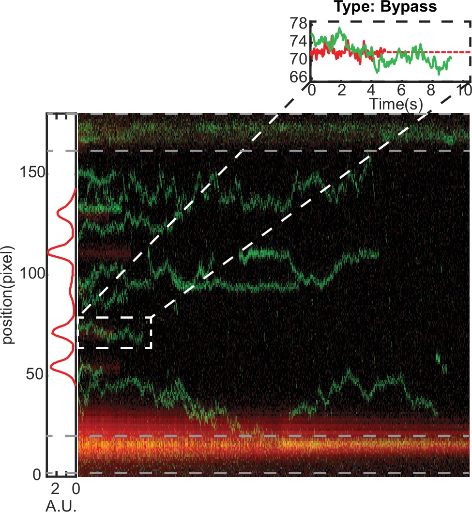
SWR1 bypassing dCas9 was a rare event.
Of 106 total colocalization events, only 3 displayed some form of bypass event. Left of the representative kymograph is a sum of the red intensity, which is used to calculate the centroid of dCas9 for colocalization analysis.
Figure 6 with 2 supplements
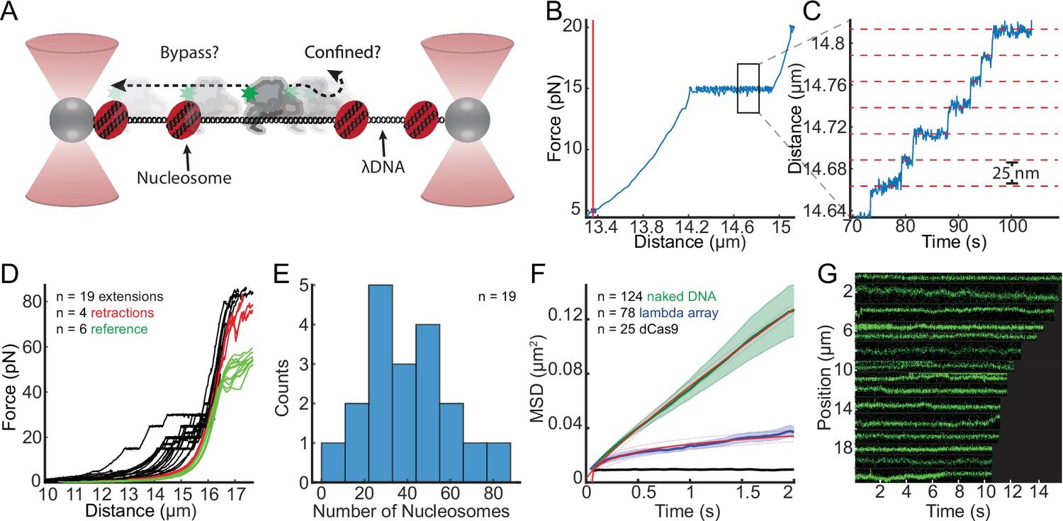
Nucleosomes confine SWR1 1D diffusion.
(A) Schematic of the experimental setup, with experimental question depicted therein. Note that diffusion is measured in the presence of 1 mM ATP and standard salt conditions (70 mM KCl). (B) Example force–distance curve showing that at 15 pN nucleosomes begin to unwrap. Vertical red line shows the length of the nucleosome array 5 pN. (C) Example unwrapping events that result in characteristic lengthening of 25 nm at this force regime. (D) Lambda nucleosome arrays extension (unwrapping) and retraction curves, with a reference naked DNA force–distance curves. Black curves are unwrapping curves where the force is clamped at either 20, 25, or 30 pN to visualize individual unwrapping events; red curves are the collapse of the DNA after unwrapping nucleosomes; green curves are reference force extension plots of lambda DNA without nucleosomes. (E) Histogram of the number of nucleosomes per array determined from the length of the array at 5 pN and the compaction ratio. (F) Mean squared displacements (MSDs) are fit over the first 2 s to MSD = Dtα, the red lines represent the fits with 95% confidence interval shown as dashed lines. SWR1 diffusing on naked DNA (green curve), on lambda nucleosome arrays (blue), and for comparison dCas9 (black). (G) Representative SWR1 particles diffusing on the nucleosome arrays are cropped and arranged by the length of the trace.
-
Figure 6—source data 1
Data underlying panels B, C, and E.
- https://cdn.elifesciences.org/articles/77352/elife-77352-fig6-data1-v2.zip
Figure 6—figure supplement 1
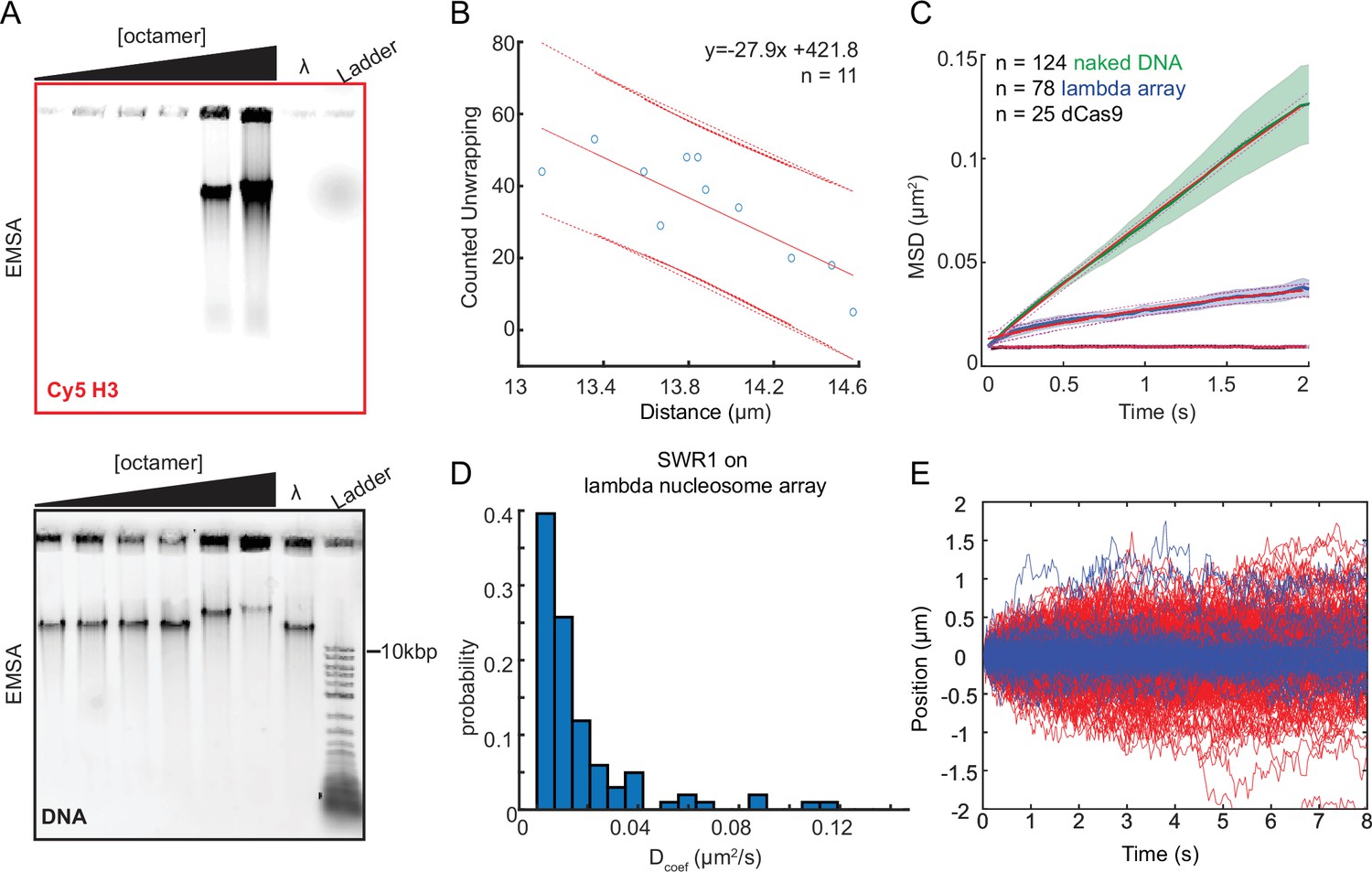
Primary lambda nucleosome array characterization.
(A) Electrophoretic mobility shift assay (EMSA) analysis of Cy5-labeled H3 octamer (~20% labeling efficiency) reconstitution to nucleosomes onto lambda DNA via salt gradient dialysis. Typhoon imager scans (top Cy5 scan, bottom SYBR Gold scan). The octamer concentrations used are as follows reported as molar ratio of octamer to DNA, from left to right: 10:1, 50:1, 100:1, 200:1, 500:1, 700:1. Lambda DNA alone is shown for reference. The 700:1 condition was selected for use in experiments. (B) The length of the nucleosome array at 5 pN and the number of unwrapping events counted are linearly related. (C) Mean squared displacement (MSD) versus time fit to y = m*(1 − exp(−b*x)) + c. For SWR1 on the lambda nucleosome array (blue), the limit approached 0.054 µm2, whereas SWR1 diffusing on lambda DNA (green) produced a limit 1.1 µm2, and dCas9 (black) produced a limit of 0.009 µm2 which is within the limits of resolution. Fits and standard error of the mean (SEM) are overlayed. (D) Histograms of diffusion coefficients extracted from individual trajectories for SWR1 diffusion on the lambda nucleosome array and in the presence of 1 mM ATP (n = 101). (E) All trajectories for SWR1 (1 mM ATP) on naked DNA (red lines) or the nucleosome array (blue lines).
-
Figure 6—figure supplement 1—source data 1
Gel images (Coomassie and Cy3 scans).
- https://cdn.elifesciences.org/articles/77352/elife-77352-fig6-figsupp1-data1-v2.zip
-
Figure 6—figure supplement 1—source data 2
Data underlying panels B and D.
- https://cdn.elifesciences.org/articles/77352/elife-77352-fig6-figsupp1-data2-v2.zip
Figure 6—figure supplement 2
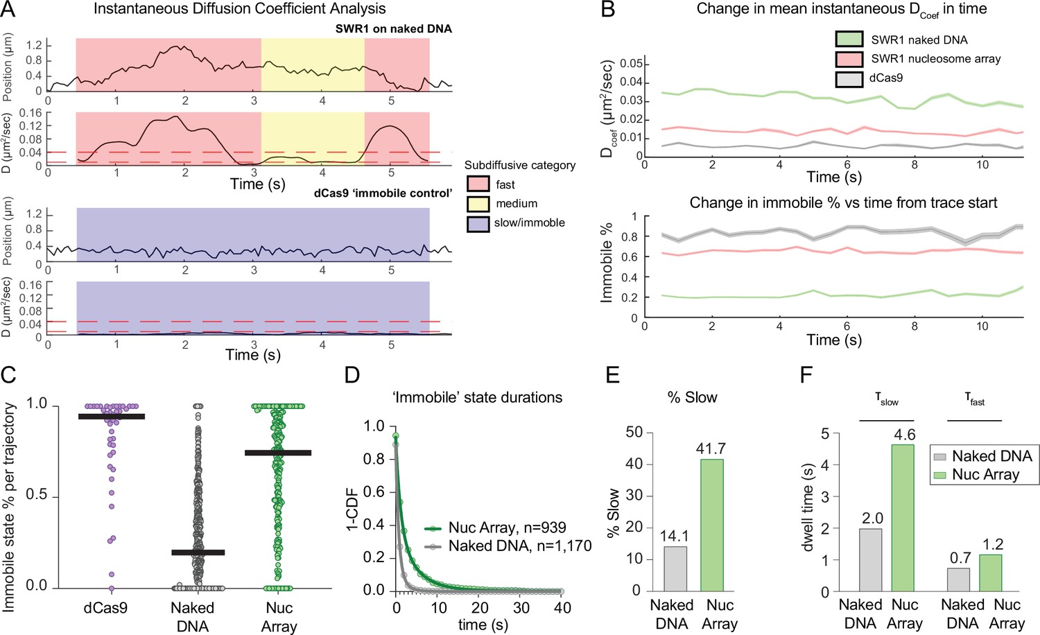
Instantaneous diffusion analysis of SWR1 diffusion on the lambda nucleosome array.
(A) Examples illustrative of the instantaneous diffusion analysis pipeline. Briefly, trajectories are subdivided into rolling windows of roughly 0.8 s in length, and diffusion coefficients are calculated using MATLAB ‘MSD analyzer’ (Tinevez, 2022). Trajectory 1 (top) is an example of SWR1 diffusion on naked DNA, where SWR1 exhibits mostly high (diffusion coefficient >0.04 µm2/s) and medium diffusion (diffusion coefficient >0.01 and <0.04 µm2/s). Trajectory 2 (bottom) is an example of dCas9 which is used as an immobile control and exhibits mostly slow/immobile instantaneous diffusion (diffusion coefficient <0.01 µm2/s). To reduce spurious detections in high/medium/low diffusion transitions caused in part by background noise, trajectories were first smoothened and only states lasting longer than 10 frames (~0.4 s) were called as real transitions. (B) (Top plot) The instantaneous diffusion coefficient averaged for all trajectories is plotted as a function of time for SWR1 on naked DNA, on the nucleosome array and for dCas9 with standard error of the mean (standard error of the mean, SEM) shown for errors. (Bottom plot) For all trajectories aligned at their starts, the percentage of traces with instantaneous diffusion characterized as immobile is plotted as a function of time with SEM shown for errors. (C) The percentage of individual traces that is slow/immobile (dCas9 with low immobile percentages represent traces collected in the presence of high background such as those collected in the dCas9 protein channel (10 mM dCas9) or near leakage from the dCas9 protein channel). Black bars indicate a median value. (D) 1-CDF dwell-time analysis of SWR1 in the slow/immobile state. Data were best fit to a double exponential decay producing a slow and fast tau value. (E) Based on the double exponential fit, the percentage of immobile events best represented by the slow tau are plotted. (F) Slow and fast tau values for SWR1 on naked DNA versus the nucleosome array.
Author response image 1
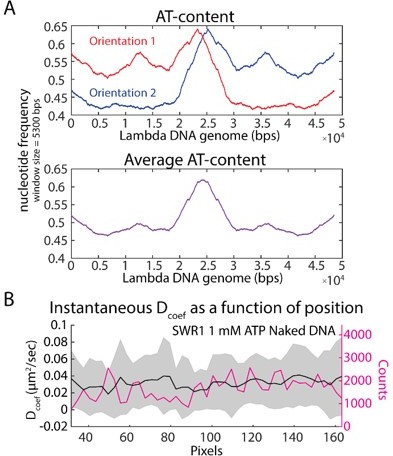
Changes in instantaneous diffusion coefficient as a function of position along the DNA substrate.
(A) The AT-content along the Λ phage genome is plotted in both orientations, revealing an asymmetric distribution of AT-content directionally across the genome. Averaging the AT-content across the two orientations shows that the center of the DNA has a slightly higher AT-content, indicating that if there is any sequence correlation to SWR1 diffusion, we may see a difference in mean diffusion coefficients at the center of the DNA (since the DNAs in this study were not intentionally oriented). (B) The instantaneous diffusion coefficient of SWR1 as a function of position along the DNA substrate. The center of the DNA substrate does not appear to exhibit any enrichment for higher or lower mobility in the SWR1 remodeler. Nonetheless, the experimental set-up would need to be further optimized to determine if there is in fact no correlation with sequence or if there is simply not enough resolution in our current set-up to discern one.
Tables
Table 1
crRNA sequences for dCas9 binding, and custom oligos sequences for DNA tethering, and dsDNA sequences used in TIRF measurements.
| ID | Identity | Sequence |
|---|---|---|
| 1 | Cas9 crRNA sequence ‘lambda 1’ | 5′-/ AltR 1/rGrGrC rGrCrA rUrArA rArGrA rUrGrA rGrArC rGrCrG rUrUrU rUrArG rArGrC rUrArU rGrCrU / AltR2/-3′ |
| 2 | Cas9 crRNA sequence ‘lambda 2’ | 5′-/ AltR 1/rGrUrG rArUrA rArGrU rGrGrA rArUrG rCrCrA rUrGrG rUrUrU rUrArG rArGrC rUrArU rGrCrU / AltR2/-3′ |
| 3 | Cas9 crRNA sequence ‘lambda 3’ | 5′-/ AltR 1/rCrUrG rGrUrG rArArC rUrUrC rCrGrA rUrArG rUrGrG rUrUrU rUrArG rArGrC rUrArU rGrCrU / AltR2/-3′ |
| 4 | Cas9 crRNA sequence ‘lambda 4’ | 5′-/AltRl /rCrArG rArUrA rUrArG rCrCrU rGrGrU rGrGrU rUrCrG rUrUrU rUrArG rArGrC rUrArU rGrCrU / AltR2/-3′ |
| 5 | Cas9 crRNA sequence ‘lambda 5’ | 5′-/AltR 1/rGrGrC rArArU rGrCrC rGrArU rGrGrC rGrArU rArGrG rUrUrU rUrArG rArGrC rUrArU rGrCrU / AltR2/-3′ |
| 6 | 3x-biotin-cos1 oligo | 5′-/5Phos/ AGG TCG CCG CCC TT/iBiodT/TT/iBiodT/TT/3BiodT/-3′ |
| 7 | 3x-biotin-cos2 oligo | 5′-/5Phos/ GGG CGG CGA CCT TT/iDigN/TT/iDigN/TT/3DigN/-3′ |
| 8 | 20 bp dsDNA | 5′-ttagcaccgggtatctccag-3′ |
| 9 | 40 bp dsdna | 5′-ttagcaccgggtatctccagatcgatgcaagggcgaattc-3′ |
| 10 | 60 bp dsdna | 5′-ttagcaccgggtatctccagatcgatgcaagggcgaattctgcagatatccatcacactg-3′ |
| 11 | 80 bp dsdna | 5′-ttagcaccgggtatctccagatcgatgcaagggcgaattctgcagatatccatcacactggcggccgctcgagcatgcat-3′ |
| 12 | 100 bp dsdna | 5′-ttagcaccgggtatctccagatcgatgcaagggcgaattctgcagatatccatcacactggcggccgctcgagcatgcatctagagggcccaattcgccc-3′ |
| 13 | 150 bp dsdna | 5′-ttagcaccgggtatctccagatcgatgcaagggcgaattctgcagatatccatcacactggcggccgctcgagcatgcatctagagggcccaattcgccctatagtgagtcgtattacaattcactggccgtcgttttacaacgtcgtga-3′ |
Table 2
Protein construct sequence.
| Identity | Sequence |
|---|---|
| Swc2 DNA-binding domain (italicized) with site of cysteine insertion in bold | HHHHHHSSGLEVLFQGPHCIRRQELLSRKKRNK RLQKGPVVIKKQKPKPKSGEAIPRSHHTHEQLN AETLLLNTRRTSKRSSVMENTMKVYEKLSKAEK KRKIIQERIRKHKEQESQHMLTQEERLRIAKETE KLNILSLDKFKEQEVWKKENRLALQKRQKQKF QPNETILQFLSTAWLMTPAMELEDRKYWQEQ LNKRDKKKKKYPRKPKKNLNLGKQDASDDKKRE |
Table 3
Summary of median diffusion coefficients as well as rejection criteria implemented per condition for particle refinement.
Also included is information regarding biological and technical replicates. ‘Trajs.’ stands for trajectories.
| Condition | Biological replicates (BR) | Min. and Max # technical replicates (TR) per BR | Total Trajs. post refine | Criteria for linear fit cutoff | Total Trajs. pre refine | Median D (μm2/s) | SEM*√(π/2) (μm2/s) | |||
|---|---|---|---|---|---|---|---|---|---|---|
| DNA or Nuc array | Protein | Nucleotide | KCl (mM) | |||||||
| DNA | SWR1 | ATP | 70 | 4 | 4–6 | 462 | p < 0.05, r2 > 0.8 | 555 | 0.024 | 0.001 |
| DNA | SWR1 | None | 70 | 4 | 4–7 | 245 | p < 0.05, r2 > 0.8 | 345 | 0.013 | 0.002 |
| DNA | SWR1 | ATPγS | 70 | 3 | 4–13 | 283 | p < 0.05, r2 > 0.8 | 367 | 0.026 | 0.002 |
| DNA | SWR1 | ADP | 70 | 3 | 5–12 | 313 | p < 0.05, r2 > 0.8 | 476 | 0.011 | 0.002 |
| DNA | SWR1 | ATP | 25 | 1 | 9 | 157 | p < 0.05, r2 > 0.8 | 171 | 0.015 | 0.001 |
| DNA | SWR1 | ATP | 200 | 1 | 8 | 131 | p < 0.05, r2 > 0.8 | 136 | 0.041 | 0.003 |
| DNA | Swc2 | None | 25 | 1 | 9 | 152 | p < 0.05, r2 > 0.8 | 200 | 0.719 | 0.069 |
| DNA | Swc2 | None | 70 | 1 | 8 | 115 | p < 0.05, r2 > 0.8 | 143 | 1.038 | 0.088 |
| DNA | Swc2 | None | 150 | 1 | 10 | 79 | p < 0.05, r2 > 0.8 | 98 | 1.549 | 0.125 |
| Nuc array | SWR1 | ATP | 70 | 4 | 4–5 | 101 | p < 0.05, r2 > 0.8 | 301 | 0.009 | 0.003 |
| DNA | dCas9 | None | 70 | 3 | 6–12 | 44 | None | 44 | 2.7 × 10⁻⁴ | 3.7 × 10⁻⁴ |
Additional files
Download links
A two-part list of links to download the article, or parts of the article, in various formats.
Downloads (link to download the article as PDF)
Open citations (links to open the citations from this article in various online reference manager services)
Cite this article (links to download the citations from this article in formats compatible with various reference manager tools)
ATP binding facilitates target search of SWR1 chromatin remodeler by promoting one-dimensional diffusion on DNA
eLife 11:e77352.
https://doi.org/10.7554/eLife.77352


