Figures and data in Dynamic readout of the Hh gradient in the Drosophila wing disc reveals pattern-specific tradeoffs between robustness and precision

Figures
Tables
Additional files

5 figures, 1 table and 1 additional file

Figures

Figure 1

Download asset Open asset

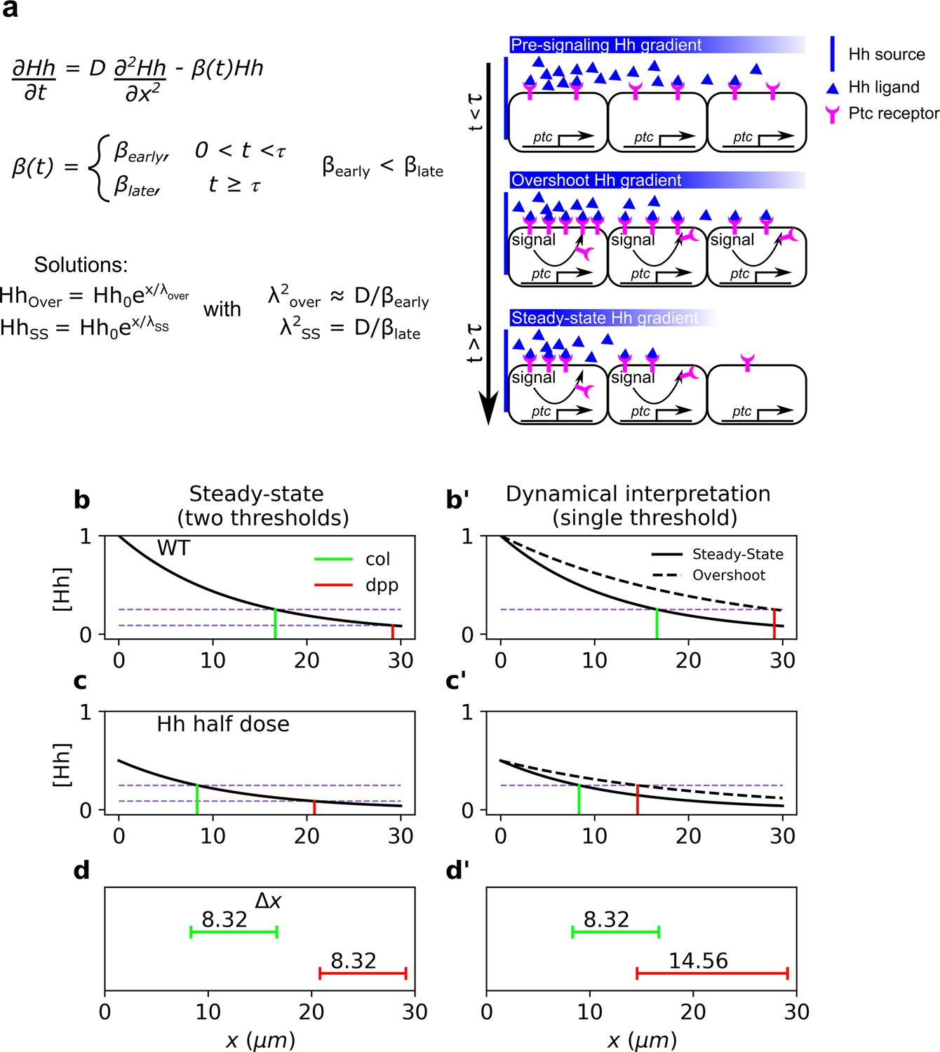
Dynamical interpretation model predicts differential robustness when morphogen dosage is reduced to half.

(a) Simple model of Hh signaling using a time-dependent step-wise degradation function. Diagrams displays a pre steady-state gradient that then retracts upon Hh-dependent *ptc* upregulation, resulting in a narrower gradient. (**b, c**) Plots of the analytical solution for the model in a using full ( $H h (x = 0) = 1$ ); (**b, b’**) or half ( $H h (x = 0) = 0.5$ ); (**c, c’**) Hh dosage. (**d, d’**) Displacements upon the above perturbation for the steady-state model with two thresholds (dotted horizontal lines corresponding to the locations of *col* and *dpp*) d; and for the dynamical interpretation model with a single-threshold readout (single dotted horizontal line) using the overshoot vs. the steady-state gradient predicts different shifts d’. The parameter values used for these plots are: $λ_{o v e r} = 21 μm$ , $λ_{S S} = 12 μm$ which approximately correspond to the anterior border positions of *col* and *dpp*, respectively. The color coding of *dpp* in red and *col* in green, will be used in the rest of the article.

Figure 1—source code 1 Code to generate Figure 1.: https://cdn.elifesciences.org/articles/85755/elife-85755-fig1-code1-v2.zip
Download elife-85755-fig1-code1-v2.zip

Figure 2

Download asset Open asset

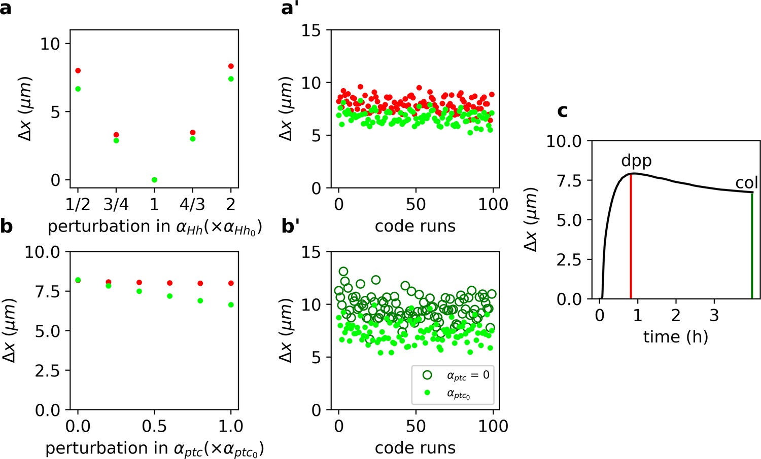
Target-specific robustness still holds in an explicit model of Hh signaling and it is dependent on Hh-dependent Ptc upregulation.

(a) $Δ x$ (defined as in Equation 1, but for the $S i g n a l$ function, see Materials and Methods) for overshoot (red) vs. steady-state (green) outputs upon different perturbations in $α_{H h}$ using the values of the parameters reported in Nahmad and Stathopoulos, 2009 (Figure 2—source code 2 and 3 and Figure 2—source data 1, 2, and 6). (a’) $Δ x$ defined and color coded as in a, for different combinations of parameter runs, when all parameters (other than $α_{H h}$ ) are varied through a random normal distribution around the mean value with a standard deviation of 10% of the mean value (Figure 2—source data 2). (b) Same as a, but for perturbations in $α_{p t c}$ (Figure 2—source data 3). (b’) Comparison of $Δ x$ for different parameters runs as in a’ for steady-state outputs (light green dots) and when $α_{p t c = 0}$ (dark green empty circles; Figure 2—source data 4). (c) $Δ x$ defined as in a, computed for the $S i g n a l$ gradient over time (Figure 2—source data 5). Red and green vertical lines indicate the overshoot and steady-state values corresponding to the anterior borders of *dpp* and *col*, respectively (Figure 2—source code 1).

Figure 2—source code 1 Code to generate Figure 2.: https://cdn.elifesciences.org/articles/85755/elife-85755-fig2-code1-v2.zip
Download elife-85755-fig2-code1-v2.zip
Figure 2—source code 2 Code to solve steady-state solution of Equation 18.: https://cdn.elifesciences.org/articles/85755/elife-85755-fig2-code2-v2.zip
Download elife-85755-fig2-code2-v2.zip
Figure 2—source code 3 Code to solve transient solution of Equations 12–17.: https://cdn.elifesciences.org/articles/85755/elife-85755-fig2-code3-v2.zip
Download elife-85755-fig2-code3-v2.zip
Figure 2—source data 1 Raw data to generate Figure 2a.: https://cdn.elifesciences.org/articles/85755/elife-85755-fig2-data1-v2.csv
Download elife-85755-fig2-data1-v2.csv
Figure 2—source data 2 Raw data to generate Figure 2a’.: https://cdn.elifesciences.org/articles/85755/elife-85755-fig2-data2-v2.csv
Download elife-85755-fig2-data2-v2.csv
Figure 2—source data 3 Raw data to generate Figure 2b.: https://cdn.elifesciences.org/articles/85755/elife-85755-fig2-data3-v2.csv
Download elife-85755-fig2-data3-v2.csv
Figure 2—source data 4 Raw data to generate Figure 2b’.: https://cdn.elifesciences.org/articles/85755/elife-85755-fig2-data4-v2.csv
Download elife-85755-fig2-data4-v2.csv
Figure 2—source data 5 Raw data to generate Figure 2c.: https://cdn.elifesciences.org/articles/85755/elife-85755-fig2-data5-v2.csv
Download elife-85755-fig2-data5-v2.csv
Figure 2—source data 6 Parameters used to solve Equations 12–17 (same values as in Nahmad and Stathopoulos, 2009).: https://cdn.elifesciences.org/articles/85755/elife-85755-fig2-data6-v2.csv
Download elife-85755-fig2-data6-v2.csv

Figure 3 with 2 supplements

Download asset Open asset

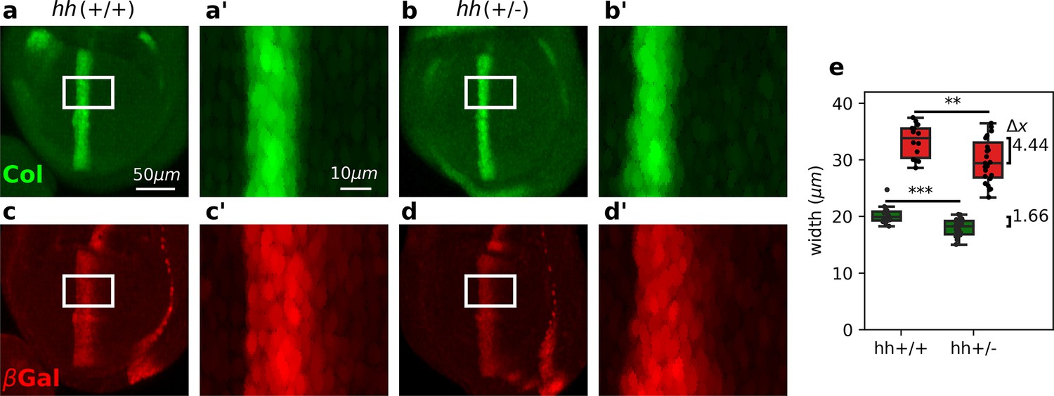
Differential robustness of Hh targets to hh dosage.

(**a-d**) Representative third-instar wild-type, hh(+/+) (**a, c**), and hh heterozygous hh(+/−) (**b, d**) wing discs immunostained with Col (**a, b**) and β-galactosidase (**c, d**) antibodies. Both hh(+/+) and hh(+/−) flies carry a transgene with a *dpp*LacZ enhancer trap, so β-galactosidase marks the pattern of *dpp* expression. The scale bars in a, a’ apply to b, b’; c, c’; and d, d’ panels, respectively. (a’**-d’**) Enlarged areas of the white boxes shown in (**a-d**). (e) Widths of the *col* and *dpp*LacZ patterns (color coded as in a–d) measured in the region marked by the white rectangle (see Figure 3—source data 1 and Figure 3—source code 1). The brackets on the right represent the difference between the medians of both groups. A non-parametric Mann–Whitney U test was applied in both cases (Figure 3—source data 1). Statistical p-values are $3.0 \times 10^{- 4}$ for Col (**) and $6.0 \times 10^{- 3}$ for *dpp*LacZ (***). hh(+/−) discs (n = 14). hh(+/+) discs (n = 23). See Figure 3—source code 1.

Figure 3—source code 1 Code to generate Figure 3.: https://cdn.elifesciences.org/articles/85755/elife-85755-fig3-code1-v2.zip
Download elife-85755-fig3-code1-v2.zip
Figure 3—source data 1 Raw data represented in Figure 3e .: https://cdn.elifesciences.org/articles/85755/elife-85755-fig3-data1-v2.csv
Download elife-85755-fig3-data1-v2.csv
Figure 3—source data 2 Raw data represented in Figure 3—figure supplement 1.: https://cdn.elifesciences.org/articles/85755/elife-85755-fig3-data2-v2.csv
Download elife-85755-fig3-data2-v2.csv

Figure 3—figure supplement 1

Download asset Open asset

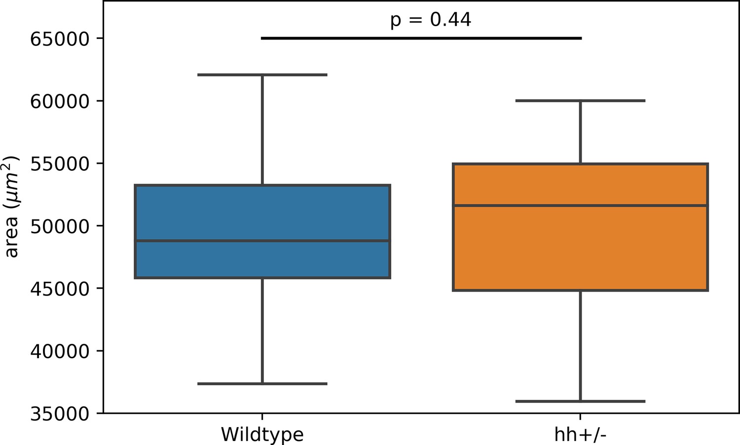
The wing disc pouch area does not change in mutant discs.

The pouch area was calculated as the area enclosed by the hinge-pouch folds. Statistical p-value after a Student t-test.

Figure 3—figure supplement 2

Download asset Open asset

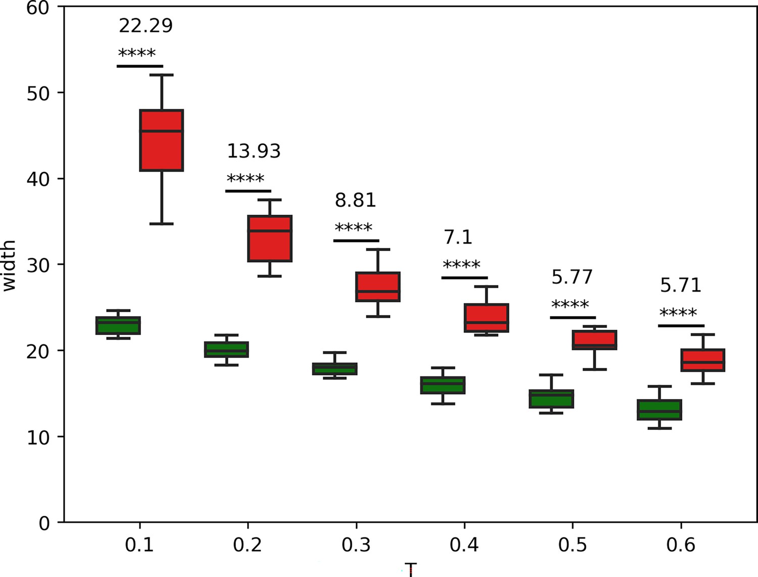
Differences in the width of col and *dpp*LacZ patterns in hh(+/+) discs at different threshold values.

Width of the gene patterns measured at different threshold concentrations measured as in Figure 3e (color coding is as in Figure 3). Numbers at the top are the differences between medians of both groups. **** indicates that p-values after a non-parametric Mann-Whitney U test are less than 0.00005.

Figure 4

Download asset Open asset

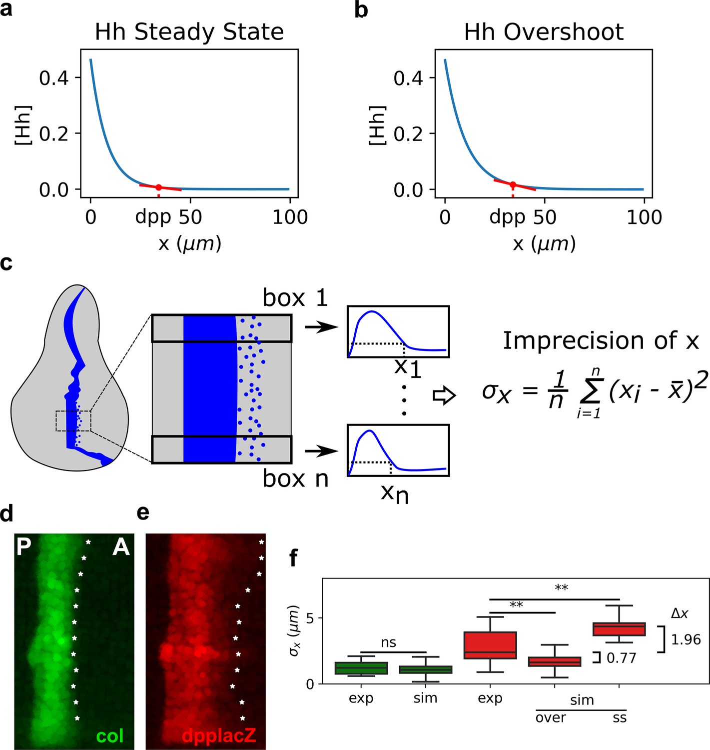
The overshoot model predicts more precision of the anterior border of *dpp* than the steady-state model.

(a, b). Representation of the steady-state (a) and overshoot (b) Hh gradients. At the location of the *dpp* anterior border, the slope of the gradient is steeper for the overshoot gradient than for the steady-state gradient. (c) Schematic representation of how we define our measure of precision for a patterning border (both in experimental and in simulated patterns). First, a box defines the region of interest (ROI) in the pattern. Then, this ROI is subdivided in $n$ boxes, each of which define a position $x_{i}$ . The measure of precision is the standard deviation of all the $x_{i}$ values. (d, e) Representative Col (d) and *dpp*LacZ (e) patterns in which the $x_{i}$ for each ROI as defined in c is measured and marked with an asterisk along the anterior border. (f) Quantification of $σ_{x}$ in several experimental (exp) and simulated (sim) patterns of *col* (green) and *dpp* (red). In the simulated patterns, noise levels are adjusted so that the distributions of *col* are not statistically significant and these noise levels are used to computed the simulated $σ_{x}$ of *dpp* as determined by the steady state (ss) or overshot (over) models. exp sample sizes as in Figure 3. sim sample sizes is n = 50 in all cases. For the statistical comparison, a Mann–Whitney U tests were applied in all cases. Statistical p-value for *col* was $p = 0.42$ . For experimental vs. overshoot *dpp*: $p = 1.0 \times 10^{- 3}$ (**), and for experimental vs. simulated steady-state *dpp*: $p = 9.0 \times 10^{- 3}$ (**).

Figure 4—source code 1 Code to generate Figure 4.: https://cdn.elifesciences.org/articles/85755/elife-85755-fig4-code1-v2.zip
Download elife-85755-fig4-code1-v2.zip
Figure 4—source data 1 Raw data represented in Figure 4f.: https://cdn.elifesciences.org/articles/85755/elife-85755-fig4-data1-v2.csv
Download elife-85755-fig4-data1-v2.csv

Figure 5

Download asset Open asset

The dynamical interpretation of the Hh gradient trades off robustness for higher precision in a target-specific manner.

In the steady-state interpretation, all the target genes are established with the same robustness ( $Δ x$ ) upon perturbations in the amount of ligand. In the overshoot model interpretation one of the target genes (red) is established with less robustness than the other (green). However, it allows the less robust gene to be defined with greater precision than the steady state would define it (compare the sharpness of the boundaries of these patterns).

Tables

Key resources table

Reagent type (species) or resource	Designation	Source or reference	Identifiers	Additional information
strain, strain background (Drosophila melanogaster)	hh(+/−) allele	Bloomington Drosophila Stock Center	1749	ry[506] hh[AC]/TM3, Sb. hh[AC] is an amorphic allele
strain, strain background (Drosophila melanogaster)	dppLacZ	Bloomington Drosophila Stock Center	12379	cn[1] dpp[10638]/CyO; ry[506]. dpp[10638] is a lacZ is a dpp enhancer trap.
antibody	anti-Col (mouse monoclonal)	Gift from M. Crozatier Vervoort et al., 1999		1:250; overnight incubation
antibody	anti-β-gal (rabbit polyclonal)	MP Biomedicals	Cat. # 55976	1:250; overnight incubation
software, algorithm	Python	this paper	pandas; numpy; OpenCV; matplotlib; seaborn; odeint; solve_bvp	Customized source codes (available from this paper)

Additional files

MDAR checklist: https://cdn.elifesciences.org/articles/85755/elife-85755-mdarchecklist1-v2.pdf
Download elife-85755-mdarchecklist1-v2.pdf

Download links

A two-part list of links to download the article, or parts of the article, in various formats.

Downloads (link to download the article as PDF)

Open citations (links to open the citations from this article in various online reference manager services)

Mendeley

Cite this article (links to download the citations from this article in formats compatible with various reference manager tools)

Rosalío Reyes
Arthur D Lander
Marcos Nahmad

(2024)

Dynamic readout of the Hh gradient in the Drosophila wing disc reveals pattern-specific tradeoffs between robustness and precision

eLife 13:e85755.

https://doi.org/10.7554/eLife.85755

Figures

Dynamical interpretation model predicts differential robustness when morphogen dosage is reduced to half.

Figure 1—source code 1

Target-specific robustness still holds in an explicit model of Hh signaling and it is dependent on Hh-dependent Ptc upregulation.

Figure 2—source code 1

Figure 2—source code 2

Figure 2—source code 3

Figure 2—source data 1

Figure 2—source data 2

Figure 2—source data 3

Figure 2—source data 4

Figure 2—source data 5

Figure 2—source data 6

Differential robustness of Hh targets to hh dosage.

Figure 3—source code 1

Figure 3—source data 1

Figure 3—source data 2

The wing disc pouch area does not change in mutant discs.

Differences in the width of col and dppLacZ patterns in hh(+/+) discs at different threshold values.

The overshoot model predicts more precision of the anterior border of dpp than the steady-state model.

Figure 4—source code 1

Figure 4—source data 1

The dynamical interpretation of the Hh gradient trades off robustness for higher precision in a target-specific manner.

Tables

Additional files

MDAR checklist

Download links

Downloads (link to download the article as PDF)

Open citations (links to open the citations from this article in various online reference manager services)

Cite this article (links to download the citations from this article in formats compatible with various reference manager tools)

Be the first to read new articles from eLife

Share this article

Cite this article

Dynamical interpretation model predicts differential robustness when morphogen dosage is reduced to half.

Figure 1—source code 1

Target-specific robustness still holds in an explicit model of Hh signaling and it is dependent on Hh-dependent Ptc upregulation.

Figure 2—source code 1

Figure 2—source code 2

Figure 2—source code 3

Figure 2—source data 1

Figure 2—source data 2

Figure 2—source data 3

Figure 2—source data 4

Figure 2—source data 5

Figure 2—source data 6

Differential robustness of Hh targets to hh dosage.

Figure 3—source code 1

Figure 3—source data 1

Figure 3—source data 2

The wing disc pouch area does not change in mutant discs.

Differences in the width of col and dppLacZ patterns in hh(+/+) discs at different threshold values.

The overshoot model predicts more precision of the anterior border of dpp than the steady-state model.

Figure 4—source code 1

Figure 4—source data 1

The dynamical interpretation of the Hh gradient trades off robustness for higher precision in a target-specific manner.

MDAR checklist

Downloads (link to download the article as PDF)

Open citations (links to open the citations from this article in various online reference manager services)

Cite this article (links to download the citations from this article in formats compatible with various reference manager tools)